Probability

While determinism was pervasive through most of the development of classical physics, it could not be maintained and uncertainty was even embraced as a central theoretical feature [79][80], as such probabilities and statistics have taken an important part among scientiﬁc modelling.

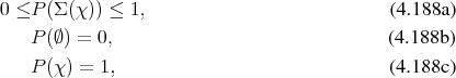
Deﬁnition 96 (Probability measure) The measure space $(χ,Σ, P)$ (Deﬁnition 92), where the measure $P$ (Deﬁnition 91) has the properties

0 ≤P (Σ(χ )) ≤ 1, (4.188a) P (∅) = 0, (4.188b) P (χ) = 1, (4.188c)

is called a probability measure. The values assigned by the measure to the subsets are called probabilities.

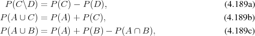
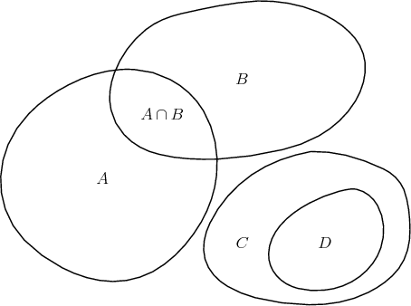
From the construction of probability as a measure it follows for a conﬁguration as shown in Figure 4.8 that

P (C ∖D ) = P (C ) − P (D ), (4.189a) P(A ∪ C ) = P (A) + P (C), (4.189b) P(A ∪ B ) = P (A) + P (B ) − P (A ∩ B ), (4.189c)

which illustrates a few basic properties of probabilities which follow directly from the use of a $σ$ -algebra (Deﬁnition 88) in the deﬁnition of a probability measure (Deﬁnition 96). The fact that the focus is not always on the introduction of a measure on a space, but rather on the resulting structure as a whole, warrants the following deﬁnition.

Figure 4.8: Sets with and without intersection.

Deﬁnition 97 (Probability space) A measure space $(χ,Σ, P )$ (Deﬁnition 92), where $P$ is a probability measure (Deﬁnition 96), is called a probability space.

Deﬁnition 98 (Random Variable) Given a probability space $(χ, Σ,μ )$ (Deﬁnition 97) and a measurable space $(χ¯, ¯Σ)$ (Deﬁnition 90) a mapping of the form

X : χ → ¯χ (4.190)

is called a random variable, if the preimages of all subspaces of the $σ$ -algebra $¯ Σ$ (Deﬁnition 88) are part of the $σ$ -algebra $Σ$

X −1(b) ∈ Σ, ∀b ∈ ¯Σ. (4.191)

The following deﬁnition facilitates the characterization of random variables and thus eases their handling.

Deﬁnition 99 (Probability distribution function) Given a random variable $X$ (Deﬁnition 98) joining the probability space $(χ,Σ, μ)$ (Deﬁnition 97) and the measurable space $¯ (¯χ, Σ)$ (Deﬁnition 90), it can be used to deﬁne a mapping $¯μ$ of the following form:

ΣX μ -----¯Σ ¯μ (4.192) | | [0;1] ¯μ = μ (X −1(b)) = μ ∘ X −1(b), ∀b ∈ ¯Σ (4.193)

$¯μ$ is an induced measure on $¯χ$ called the probability distribution function $P$ , also called the cumulative probability function.

A concept closely related to the probability distribution function which allows for a local description, is given next.

Deﬁnition 100 (Probability density function) Given a probability distribution function $P$ (Deﬁnition 99) the probability density function $p$ is deﬁned as satisfying the relation

∫ ∫ P(X ) = ¯μ(X ) = X−1(¯χ)dμ = χ¯pdμ¯. (4.194)

Deﬁnition 101 (Expectation value) Given a probability space $(χ,Σ, μ)$ (Deﬁnition 97) and a random variable $X$ (Deﬁnition 98) the expectation value $⟨X ⟩$ is deﬁned by the prescription

∫ ⟨X ⟩ = Xd μ. (4.195) χ

In case a probability distribution (Deﬁnition 100) is given, the expectation value also takes the shape

Among the inﬁnite number of conceivable probability measures a few select are provided in the following, since they have uses in Section 7.2.

Deﬁnition 102 (Uniform distribution) A probability distribution $P$ (Deﬁnition 99) on a space $χ$ , which has a constant probability density function $p$ (Deﬁnition 100) is called a uniform distribution.

p = const (4.197) P(χ ) = 1 (4.198)

Deﬁnition 103 (Exponential distribution) The exponential distribution is associated to the cumulative distribution function (Deﬁnition 99).

−λx P (x) = 1 − e , ∀x ≥ 0 (4.199)

From this the probability density function $p$ (Deﬁnition 100) can be derived to read

p(x) = λe−λx, ∀x ≥ 0 (4.200)

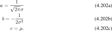
Deﬁnition 104 (Normal distribution) A probability distribution function $P$ with a probability density function of the shape

p(x) = aeb(x− c)2, a, b,c ∈ ℝ, b < 0 (4.201)

is called normal or Gaußian. The factors are often associated the variance $2 σ$ , and the mean value $μ$ by the expressions

1 a = √----- (4.202a) 2π σ -1-- b = − 2σ2 (4.202b) c = μ. (4.202c)

If this is the case and furthermore $μ = 0$ and $2 σ = 1$ , it is commonly called standard normal distribution.

The importance of the normal distribution can be linked to the central limit theorem, which states that a series of independently distributed random variables approaches normal distribution in the limit and thus can be approximated using normal distribution.

The normal distribution can also be used to deﬁne other distributions as in the following.

Deﬁnition 105 (Lognormal distribution) A random variable $Y$ , which is obtained from a normally distributed (Deﬁnition 104) variable $X$ by

X Y = e (4.203)

is called log-normally distributed.

4.10 Probability