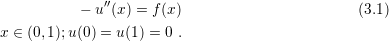
As a starting point, consider the boundary value problems (BVP) described by
Additionally, define a linear space  as:
as:
V = {v: continous functions in [0,1] with v’ piecewise continous and
bounded in [0,1], and v(0)=v(1)=0}
Along this session, it will be shown how the space  can be used to reformulate the
problem (3.1). From this new version, a numerical method will be developed based on
the particular definition of
can be used to reformulate the
problem (3.1). From this new version, a numerical method will be developed based on
the particular definition of  , in order to obtain an approximate solution of
(3.1).
To begin, take an element of the space
, in order to obtain an approximate solution of
(3.1).
To begin, take an element of the space  , multiply by (3.1) and integrate over the entire
domain as in
, multiply by (3.1) and integrate over the entire
domain as in
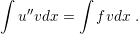 | (3.2) |
 is known as a test function. Initially, it is not clear how (3.2) can help
to solve (3.1), but it provides a different view of the problem (3.1). Indeed, it is
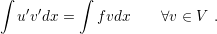
possible to simplify (3.2) by integrating the left hand side by parts, according
to
is known as a test function. Initially, it is not clear how (3.2) can help
to solve (3.1), but it provides a different view of the problem (3.1). Indeed, it is
possible to simplify (3.2) by integrating the left hand side by parts, according
to
 | (3.3) |
 | (3.4) |