In macroscopic semiconductor device modeling, Poisson's equation and the
continuity equations play a fundamental role. Poisson's equation, one of the
basic equations in electrostatics, is derived from the Maxwell's equation
![]() and the material relation
and the material relation
![]()
![]() stands for the electric displacement field,
stands for the electric displacement field,
![]() for the electric field,
for the electric field,
![]() is the charge density, and
is the charge density, and
![]() is the permittivity tensor. Using the
electrostatic potential
is the permittivity tensor. Using the
electrostatic potential ![]() with
with
![]() leads to Poisson's
equation
leads to Poisson's
equation
In semiconductors the charge density is commonly split into fixed charges which
are in particular ionized acceptors
![]() and donors
and donors
![]() and into free
charges which are electrons
and into free
charges which are electrons ![]() and holes
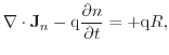
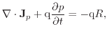
and holes ![]() Including the acceptors, donors, electrons, and holes into (4.1),
Poisson's equation can be written as
Including the acceptors, donors, electrons, and holes into (4.1),
Poisson's equation can be written as
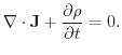
The continuity equation, can be also derived from Maxwell's equations and reads
A semiclassical description of carrier transport is given by Boltzmann's
transport equation (BTE) which describes the evolution of the distribution
function in the six-dimensional phase space (![]()
![]()
![]()
![]()
![]()
![]() ). Unfortunately, analytical solutions exist only for very simple
configurations. One popular approach for solving the BTE in arbitrary
structures is the Monte Carlo method [122] which gives highly
accurate results. However, due to the statistical nature of the Monte Carlo
method solutions are computationally very expensive. Due to the good agreement
with experiments [123] results are often used as reference for
the evaluation of simpler models. Alternatively, the spherical harmonics
expansion (SHE) method as a deterministic numerical solution method of the BTE
was presented already in the 1960s [124]. However, it has just been
recently, that an efficiently use on real devices has been realized
[125].
). Unfortunately, analytical solutions exist only for very simple
configurations. One popular approach for solving the BTE in arbitrary
structures is the Monte Carlo method [122] which gives highly
accurate results. However, due to the statistical nature of the Monte Carlo
method solutions are computationally very expensive. Due to the good agreement
with experiments [123] results are often used as reference for
the evaluation of simpler models. Alternatively, the spherical harmonics
expansion (SHE) method as a deterministic numerical solution method of the BTE
was presented already in the 1960s [124]. However, it has just been
recently, that an efficiently use on real devices has been realized
[125].
Device simulations on an engineering level require simpler transport equations which can be solved for complex structures within reasonable time. One method to perform this simplification is to consider only moments of the distribution function [126]. Depending on the number of moments considered in the model, different transport equations can be derived. The use of the first two moments, leads to the well known drift-diffusion model, a widely used approach for modeling carrier transport.
Beside the derivation of the drift-diffusion by the method of moments
[11], it is also possible using basic principles of
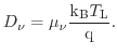
irreversible thermodynamics [127]. The resulting electron and
hole current relations contain at least two components caused by carrier drift
and carrier diffusion. Additionally, the gradient of the lattice temperature
(
![]() ) acts as a driving force on the free carriers leading to
[128]
) acts as a driving force on the free carriers leading to
[128]
The equations (4.7) and (4.8) together with (4.5), (4.6), and (4.2) form the drift-diffusion model which was first presented by Van Roosbroeck in the year 1950 [129]. Rigorous derivations from the BTE show that many simplifications are required to obtain the drift-diffusion equations as will be shown. Simplifications include, for example, the assumption of a single parabolic band structure and the cold Maxwellian carrier distribution function. This assumes the carrier temperature equal to the lattice temperature. Nevertheless, due to its simplicity and its excellent numerical properties, the drift-diffusion equations have become the workhorse for most TCAD applications.
To obtain a better approximation of the BTE, higher-order transport models can be derived using more than just the first two moments [130]. The most prominent models beside the drift-diffusion model are the energy-transport/hydrodynamic models which use three or four moments. These models are based on the work of Stratton [131] and Bløtekjær [132]. A detailed review is given in [15]. In addition to the quantities used in the drift-diffusion model, the energy flux and the carrier temperatures are introduced as independent variables. Also new balance and flux equations are required, which introduce additional transport parameters. The carrier energy distribution function is here modeled using the heated Maxwellian distribution. Modeling of carrier mobility and impact-ionization benefit from more accurate models based on the carrier temperatures rather than the electric field. This advantage is caused by the non-local behavior of the average energy with respect to the electric field and becomes especially relevant for small device structures. This context is explained in Fig. 4.2.
![\includegraphics[width=0.51\textwidth]{figures/nonlocal.eps}](img185.png)
![\includegraphics[width=0.51\textwidth]{figures/distr.eps}](img186.png)
|
More detailed examinations in the far sub-micron area show that describing the energy distribution function using only the carrier concentration and the carrier temperature is still not sufficient for specific problems which depend on high energy tails (see Fig. 4.2). Hot carrier modeling in small structures, for example, which is based on accurate modeling of the high-energy part of the distribution function would require more complex models. Also the reliability modeling benefits of the detailed knowledge of the distribution function (more on this is highlighted in Chapter 6). One method for improving the approximation of the distribution function is the six moments method [134]. It introduces the kurtosis, which is the deviation of the distribution function from the heated Maxwellian.
It is evident that higher-order transport models give a closer solution of the BTE and therefore lead to a better agreement between simulation results and measurements of real devices. This effect is especially relevant for small structures, where non-local effects gain importance (see Fig. 4.2). Simulation results with drift-diffusion in deep sub-micrometer structures therefore seem to be very questionable [135].
The high-voltage devices considered in this work are relatively large. Hence, a rather high number of mesh points is required for a proper discretization. In combination with more elaborative transport equations, this leads to a higher computational time. Additionally, the convergence properties degrade significantly for higher moments models [136]. However, the relatively large dimensions of the high-voltage devices justify the use of the drift-diffusion model in this work.
In case advanced transport models have to be solved in complex devices, it is also possible to combine different transport equations in one simulation. To accomplish this, the semiconductor domain must be partitioned into separate segments. One segment must contain the critical areas, e.g. the channel area. Hence, the higher-order transport equations are solved for this segment, and the drift-diffusion model is used for the remaining ones. Here, it is essential to define proper boundary conditions between the segments [137].