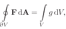
The discretization of the partial differential semiconductor equations in space and time is required to obtain difference equations which can be solved using numerical methods. A common approach for the discretization of the differential equations is the box discretization or box integration method [259,12], also known as the finite volume method.
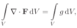
The box discretization method reformulates the equations based on this Voronoi tessellation and can be equally used in two- and three-dimensional simulation domains. Since the two-dimensional devices have a specified width which acts as a multiplier, all boxes are considered as volumes and the box boundary elements are considered as surfaces. The basic method of the box discretization concerns the divergence operator in the form
 |
(7.2) |
| (7.5) |
![\includegraphics[width=0.45\textwidth]{figures/box_int.eps}](img649.png)
|
The physical equations that describe semiconductor devices are laws of
conservation. The derivation of the box discretization method is inherently
conservative [260]. The box discretization scheme is,
therefore, widely used in semiconductor device simulations
[12]. In drift-diffusion simulations, the differential equations that have
to be solved are Poisson's equation (4.1) and the current
continuity equations (4.5) and (4.6). The flux quantities
![]() introduced in (7.1) are the dielectric flux density
introduced in (7.1) are the dielectric flux density
![]() for Poisson's equation and the current densities
for Poisson's equation and the current densities
![]() for the continuity equation, respectively. The generation terms
for the continuity equation, respectively. The generation terms ![]() in
(7.1) are the charge density
in
(7.1) are the charge density ![]() and the carrier
generation/recombination rates
and the carrier
generation/recombination rates ![]() /
/![]() respectively.
respectively.
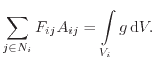
A considerable advantage of the box discretization method is that the only
information required is the unstructured neighborhood information. This
neighborhood information consists basically of two lists. First, a list of all
boxes in the simulation domain, together with their center points (![]() ),
i.e. the vertices, and the box volumes (
),
i.e. the vertices, and the box volumes (![]() ). Second, a list of all edges
connecting the vertices, together with the edge length (
). Second, a list of all edges
connecting the vertices, together with the edge length (![]() ), i.e. the
distance between the vertices, and the common surface between the neighboring
boxes (
), i.e. the
distance between the vertices, and the common surface between the neighboring
boxes (
![]() ). It has to be noted that no more information about the elements
is necessary for the evaluation of (7.4), which makes the box
discretization independent of the box shape, including its dimensionality. This
makes this scheme very straightforward to implement and a dimensional
independent set-up of the simulator can be realized.
). It has to be noted that no more information about the elements
is necessary for the evaluation of (7.4), which makes the box
discretization independent of the box shape, including its dimensionality. This
makes this scheme very straightforward to implement and a dimensional
independent set-up of the simulator can be realized.
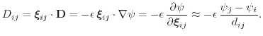
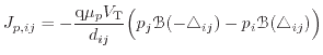
The calculation of the one-dimensional projection of the flux on the edge
depends on the type of the differential equation. For the dielectric flux
density
![]() in Poisson's equation the flux from box
in Poisson's equation the flux from box ![]() to box
to box ![]() along the
connecting edge through the common boundary area
along the
connecting edge through the common boundary area
![]() is
is ![]() This
density is commonly approximated using the directional derivative of the
electrostatic potential:
This
density is commonly approximated using the directional derivative of the
electrostatic potential:
For the current densities
![]() of the carrier type
of the carrier type ![]() the
discretization of
the
discretization of
![]() is not as straightforward. Insertion of the
drift-diffusion current relations from equations (4.7) and (4.8) in the
continuity equations (4.5) and (4.6) results in a second
order parabolic partial differential equation. Using a simple finite difference
approach like in (7.6) leads to numerical oscillations if
the drift term dominates over the diffusion term [261]. Very fine
meshes would be necessary to stabilize the system. A stable discretization can
be obtained using the Scharfetter-Gummel method [39]
instead. Here, the drift-diffusion current equations (4.7) and (4.8) are
used to solve the one-dimensional carrier concentrations,
is not as straightforward. Insertion of the
drift-diffusion current relations from equations (4.7) and (4.8) in the
continuity equations (4.5) and (4.6) results in a second
order parabolic partial differential equation. Using a simple finite difference
approach like in (7.6) leads to numerical oscillations if
the drift term dominates over the diffusion term [261]. Very fine
meshes would be necessary to stabilize the system. A stable discretization can
be obtained using the Scharfetter-Gummel method [39]
instead. Here, the drift-diffusion current equations (4.7) and (4.8) are
used to solve the one-dimensional carrier concentrations, ![]() and
and ![]() respectively, along the edge. The boundary conditions of the carrier
concentrations are given using the values at the corresponding vertices
respectively, along the edge. The boundary conditions of the carrier
concentrations are given using the values at the corresponding vertices ![]() and
and
![]() The values of
The values of ![]() and
and ![]()
![]() and
and ![]() and
and ![]() are considered constant along the edge. Solving this one-dimensional
differential equation results in
are considered constant along the edge. Solving this one-dimensional
differential equation results in
| (7.9) |
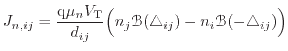
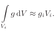
Up to now, the generation term ![]() on the right hand side of
(7.4), which is the charge density
on the right hand side of
(7.4), which is the charge density ![]() in Poisson's equation
and the carrier generation and recombination rate in the carrier equations, was
only represented as an integral in continuum space. Most implementations
calculate this integral by partitioning the box into pieces and adding the
contributions to the integral of the box. Three different methods are
considered in this work, each partitioning the Voronoi box differently. For the
first assumption, the box is not split and the generation is considered
constant over the whole box volume, as it is depicted in
Fig. 7.6(a). This approach reduces the integral term of
(7.4) to a simple product [12,262] which
reads
in Poisson's equation
and the carrier generation and recombination rate in the carrier equations, was
only represented as an integral in continuum space. Most implementations
calculate this integral by partitioning the box into pieces and adding the
contributions to the integral of the box. Three different methods are
considered in this work, each partitioning the Voronoi box differently. For the
first assumption, the box is not split and the generation is considered
constant over the whole box volume, as it is depicted in
Fig. 7.6(a). This approach reduces the integral term of
(7.4) to a simple product [12,262] which
reads
![\includegraphics[width=\textwidth]{figures/box_html_eps}](img672.png)
|
This formulation perfectly fits to the box discretization method, because it only requires quantities which are stored on vertices and the only geometry information needed is the unstructured neighborhood information. This makes the assembling procedure of (7.10) very simple. MINIMOS-NT [120], for example, is one simulation tool using this technique. As will be discussed in Section 7.3, the calculation of vector quantities is somewhat more involved in this approach than for the other methods.
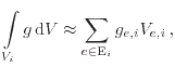
Another approach for assembling the generation integral is to assume the
generation rate to be constant within one mesh element. In this case, the
integral for one box volume is assembled using contributions from all adjacent
elements ![]() Using the naming conventions from Fig. 7.6(b), this
reads
Using the naming conventions from Fig. 7.6(b), this
reads
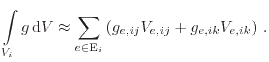
The third approach in this classification is depicted in Fig. 7.6(c). This approach was presented for triangles only [263], but extensions to tetrahedra are possible. Here, each triangle is split into three different regions associated with the three edges. In each of them, a generation term is estimated, and two of them contribute to the sum of one box. Therefore, the summation for the generation integral of the box requires to consider two contributions per element:
The box method is used in most numerical device simulation environments as it
is particle conservative and has proven to deliver good results, is numerically
very stable, and is relatively simple to implement. Problems arise when the
Delaunay criterion is violated. This leads to obtuse elements which degenerate
the accuracy due to negative flux areas
![]() [267,264]. Also, use of the one-dimensional
Scharfetter-Gummel discretization to solve multiple dimensional problems leads
to the crosswind diffusion effect resulting in artificial current components
perpendicular to the actual current direction [268]. The accuracy of
the discretization also degrades if triangles are aligned with the hypotenuse
along the current flow. As depicted in Fig. 7.7, a vanishing
boundary area
[267,264]. Also, use of the one-dimensional
Scharfetter-Gummel discretization to solve multiple dimensional problems leads
to the crosswind diffusion effect resulting in artificial current components
perpendicular to the actual current direction [268]. The accuracy of
the discretization also degrades if triangles are aligned with the hypotenuse
along the current flow. As depicted in Fig. 7.7, a vanishing
boundary area ![]() leads according to (7.4) to a vanishing
contribution of the current along this edge.
A zig-zag characteristic of the discretized current is the result. There have
been many proposals for more accurate discretizations (e.g. Patil in
[267]). Some focus on the extension of the one-dimensional to a
two-dimensional Scharfetter-Gummel current discretization
[269,270]. But none of these extensions is as universal
to use as the box integration method which is dimension independent and can be
used for structured and unstructured meshes alike.
leads according to (7.4) to a vanishing
contribution of the current along this edge.
A zig-zag characteristic of the discretized current is the result. There have
been many proposals for more accurate discretizations (e.g. Patil in
[267]). Some focus on the extension of the one-dimensional to a
two-dimensional Scharfetter-Gummel current discretization
[269,270]. But none of these extensions is as universal
to use as the box integration method which is dimension independent and can be
used for structured and unstructured meshes alike.
![\includegraphics[width=0.45\textwidth]{figures_book/tri_surface.eps}](img678.png) |