In order to calculate the subband structure in the inversion layer the Schrödinger equation
and the Poisson equation have to be considered as a coupled system of differential
equations, which has to be solved self-consistently by numerical
methods [Vasileska00]. The energy levels  and envelope wavefunctions
 are determined by a solution of the effective Schrödinger equation
![$\displaystyle [T-e\Phi (z)]\psi = E\psi\ ,$](img692.png) |
(4.1) |
where  is the electrostatic potential and
  is the operator for
the kinetic energy. The electrostatic potential determining the shape
of the potential well is the solution of the Poisson equation
is the operator for
the kinetic energy. The electrostatic potential determining the shape
of the potential well is the solution of the Poisson equation
![$\displaystyle \nabla^2 \Phi = - {\frac{e}{\ensuremath{\kappa_\mathrm{si}}{}}} [N_{\mathrm{dop}}(z) + p(z) - n(z)]\ .$](img694.png) |
(4.2) |
Here,
 is the doping profile in the semiconductor, and
 and
and  denote the hole and electron concentration, respectively. The
boundary conditions for the potential are
denote the hole and electron concentration, respectively. The
boundary conditions for the potential are
 for the bulk interface and
 |
(4.3) |
for the Si-SiO interface. In (4.3)
 denotes the dielectric permittivity of the insulating
layer and
denotes the dielectric permittivity of the insulating
layer and
 that of the
semiconductor. Assuming the effective mass approximation, the kinetic
energy operator in (4.1) can be written as
that of the
semiconductor. Assuming the effective mass approximation, the kinetic
energy operator in (4.1) can be written as
 |
(4.4) |
where
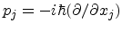 denotes the momentum operator, and
 is the reciprocal effective mass tensor. A coordinate system is
chosen such that the
is the reciprocal effective mass tensor. A coordinate system is
chosen such that the  axis is normal to the semiconductor-insulator
interface.
axis is normal to the semiconductor-insulator
interface.
Figure 4.1:
Angles  and
and  with respect to
the coordinate system which diagonalizes the inverse effective mass tensor.
with respect to
the coordinate system which diagonalizes the inverse effective mass tensor.
|
|
The conduction band valleys of semiconductors are typically oriented along high
symmetry lines of the first Brillouin zone. To calculate the subband structure
for any substrate orientation, it is necessary to introduce a unitary
transformation from the crystallographic system  to the interface
coordinate system. The momentum operator and the reciprocal effective mass
tensor in the interface coordinate system are transformed as
to the interface
coordinate system. The momentum operator and the reciprocal effective mass
tensor in the interface coordinate system are transformed as
Here,  are the elements of a unitary matrix,
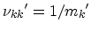 ,
where
,
where  denote the principal effective masses of the constant-energy
ellipsoid in the semiconductor. The unitary transformation matrix from the
crystallographic coordinate system to the interface coordinate system is given
by
denote the principal effective masses of the constant-energy
ellipsoid in the semiconductor. The unitary transformation matrix from the
crystallographic coordinate system to the interface coordinate system is given
by
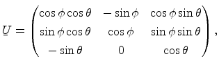 |
(4.7) |
and involves a rotation of about the  axis followed by a subsequent
rotation of about the new
axis followed by a subsequent
rotation of about the new  axis (compare
Figure 4.1). The direction of the new axis after the
two rotations is thus given by the last column of
axis (compare
Figure 4.1). The direction of the new axis after the
two rotations is thus given by the last column of
 ,
,
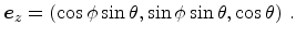 |
(4.8) |
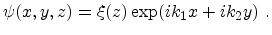
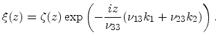
Since the potential is assumed to be a function of only, it is possible to
the separate the trial solution of (4.1) into a -dependant factor
 , and a plane wave factor representing free motion in the
  plane
[Stern67]
plane
[Stern67]
 |
(4.9) |
The functions  must satisfy the equation
 |
(4.10) |
where
 |
(4.11) |
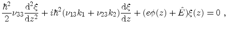
Following Stern and Howard [Stern67], the first derivative in the above
equation can be eliminated using the substitution4.1
 |
(4.12) |
The differential equation for  takes the form
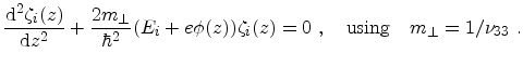 |
(4.13) |
The eigenfunctions being subject to the boundary conditions
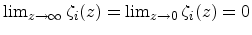 and
the eigenvalues of (4.13) are labeled by a subscript
and
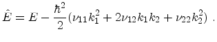
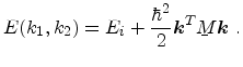
the eigenvalues of (4.13) are labeled by a subscript  . The energy
spectrum is given by
. The energy
spectrum is given by
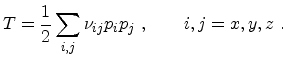
![$\displaystyle E(k_1,k_2)= E_i + \frac{\hbar^2}{2}\left [ \left ( \nu_{11} - \fr...
...k_1k_2 + \left ( \nu_{22} - \frac{\nu_{23}^2}{\nu_{33}}\right ) k_2^2 \right ].$](img729.png) |
(4.14) |
and represents constant-energy ellipses above the minimum energy  . The
fact that is independent of
. The
fact that is independent of  and
and  is a result of the boundary
condition
is a result of the boundary
condition
 . The energy levels for a given value of
  generate a set of subband minima called subband ladder. Since the value of the
quantization mass depends on the substrate orientation, so do the number and
the degeneracy of the subband ladders. Obviously, if conduction band valleys have
the same orientation with respect to the surface, these valleys belong to the
same subband ladder. Because of the kinetic energy term (4.4) in
the Schrödinger equation the valleys with the largest quantization mass have the
lowest energy. Following a widely used convention, the subbands belonging to
the ladder lowest in energy are labeled
generate a set of subband minima called subband ladder. Since the value of the
quantization mass depends on the substrate orientation, so do the number and
the degeneracy of the subband ladders. Obviously, if conduction band valleys have
the same orientation with respect to the surface, these valleys belong to the
same subband ladder. Because of the kinetic energy term (4.4) in
the Schrödinger equation the valleys with the largest quantization mass have the
lowest energy. Following a widely used convention, the subbands belonging to
the ladder lowest in energy are labeled
 , those of the second
ladder
, those of the second
ladder
 , the third ladder
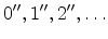 , and so
on [Ando82].
, and so
on [Ando82].
The principal effective masses
 and
and
 , associated with motion parallel to the surface can be
deduced from (4.14). This equation represents an ellipse whose principal
axes are not parallel to and . Introducing the matrix
, associated with motion parallel to the surface can be
deduced from (4.14). This equation represents an ellipse whose principal
axes are not parallel to and . Introducing the matrix
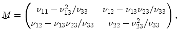 |
(4.15) |
equation (4.14) can be written as
 |
(4.16) |
The inverse effective masses
 and
and
 are the eigenvalues of
 and can be
calculated by solving the secular equation
and can be
calculated by solving the secular equation
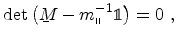 |
(4.17) |
where
 denotes the two dimensional unity matrix.
Subsections
E. Ungersboeck: Advanced Modelling Aspects of Modern Strained CMOS Technology
![\includegraphics[scale=1.3, clip]{inkscape/coordinateRotation_2.eps}](img705.png)