Next: 2. The Three-Dimensional Electron
Up: Dissertation Martin-Thomas Vasicek
Previous: List of Figures
Subsections
THE FUNDAMENTAL equation of semi-classical transport is Boltzmann's
transport equation (BTE). A common transport model, which can be easily
derived from BTE is the drift-diffusion model, which is the workhorse of
today's Technology Computer Aided Design (TCAD) tools. However, driven
by Moore's law, the device dimensions of modern semiconductors decrease into
the deca-nanometer regime following that the drift-diffusion model gets more and
more inaccurate. A solution is to use more sophisticated models based
on BTE like the Monte Carlo approach
(MC) [22,23,24,25].
The disadvantage of the MC technique is it's high computational effort due
to the statistical approach and hence rather less suitable for engineering
applications. However, the results obtained from the MC simulation method
are often in a good agreement with the experiment [1] and frequently used as a benchmark for other simpler models.
For engineering purposes, higher-order macroscopic models based on the method
of moments such as the hydrodynamic, six moments, or even higher-order models
are adequate approaches for modeling sub-microscopic
devices [21]. A
detailed discussion will follow in the sequel.
Another promising approach for solving the BTE is the method of spherical
harmonics [26]. The underlying idea is to expand the
distribution function into spherical harmonics and exploit the orthogonality of
the basis (see Section 1.4.5).
Since the BTE is a semi-classical equation including both Newton
mechanics and the quantum mechanical scattering operator, transport models, as
explained above, are only valid in a certain regime, where quantum effects like
source to drain tunneling play only a negligible
role (see Fig. 1.1) [27,28,29].
Figure 1.1:
Hierarchy of transport models
|
|
In order to cover the range of gate lengths below
 , where
source to drain tunneling plays an important role, several quantum mechanical
approaches have been developed. The Landauer-Büttiker approach is valid
in a ballistic regime, where the carriers are not affected by
scattering [30]. This approach is based on a generalization of
the conduction characterized by the transmission and reflection of the
carriers. However, in general, transport models in the deca-nanometer regime are
based on the fundamental equation of quantum mechanics, the Schrödinger
equation (see Fig. 1.1).
, where
source to drain tunneling plays an important role, several quantum mechanical
approaches have been developed. The Landauer-Büttiker approach is valid
in a ballistic regime, where the carriers are not affected by
scattering [30]. This approach is based on a generalization of
the conduction characterized by the transmission and reflection of the
carriers. However, in general, transport models in the deca-nanometer regime are
based on the fundamental equation of quantum mechanics, the Schrödinger
equation (see Fig. 1.1).
The non-equilibrium Green's function (NEGF) formalism is a powerful
method to handle open quantum systems [31]. The method can be used
both in a ballistic and a scattering dominated regime (see Section 1.3.1). If
the mean free path of the carriers is smaller than the device size, the system
is in a scattering dominated regime, while if the mean free path is longer than
the device the system can be described ballistically.
Other quantum approaches are based on a MC solution of the Wigner
equation [32]. The advantage, compared to NEGF is that the
methods comprise the coordinates and the momentum as the degree of freedom. In
the NEGF method, the additional degree of freedom is the energy. In the
classical limit of Wigner Monte Carlo, the results converge to the Monte Carlo results
based on the BTE. A drawback of the Wigner equation is that the
equation is not positive definite. In literature, this is known as the
negative-sign problem [33]. This method can be used as well in
the ballistic as in the scattering dominated regime.
The so called Pauli Master equation is derived from the Liouville von Neumann
equation. The Liouville von Neumann equation describes the quantum evolution of the
density matrix and forms the fundamental equation for the Pauli master
equation. The Pauli master equation is a frequently used model of
irreversible processes in simple quantum systems and can be used in the
ballistic and in the scattering dominated
regions [34,35].
The Lindblad master equation, the last point of the mentioned quantum models
in Fig. 1.1, is the most general form of the Liouville von Neumann
equation. It characterizes the non-unitary evolution of the density matrix. The
elements of the density matrix are trace preserving and
positive [36,37,38].
Other methods to cover gate lengths below the semi-classical regime are quantum
macroscopic transport models. These models as the quantum drift-diffusion
model or the quantum hydrodynamic model can be derived from the Schrödinger
equation using the so called Madelung
transformation [39]. A discussion will follow
in Section 1.3.3.
All models have Poisson's equation in common, which describes the
electrostatics of the system. For a new simulation strategy, it is also
important to investigate the underlying material and to compare the simulation
results with measurement data.
The basic equations of quantum and classical device simulations, namely
Poisson's equation, the Schrödinger equation, and the BTE with its
solution, the distribution function, are derived and discussed in this section.
1.1.1 Derivation of Poisson's Equation
Poisson's equation is the basic equation of electrostatics [40,41]. It can
be derived inserting the definition of the electric field

into the second Maxwell equation
Here,
 denotes the electrostatic potential,
 represents
the charge density, and
represents
the charge density, and
 is the electric displacement field defined
as
is the electric displacement field defined
as
Combining equation (1.1) with (1.2) yields Poisson's equation
whereby
can be expressed as
 , and
, and
 denote the holes and the electron concentration, respectively,
whereas
denote the holes and the electron concentration, respectively,
whereas
 and
and
 are the concentration of acceptors and
donors [42]. Inserting (1.5) into (1.6)
yields
are the concentration of acceptors and
donors [42]. Inserting (1.5) into (1.6)
yields
A complete description of transport within a device is achieved solving
Poisson's equation self-consistently with the appropriate formulation of
carrier transport within the semiconductor.
1.1.2 Schrödinger-Poisson System
In classical physics, the evolution in time and space of an ensemble of
particles can be characterized using Newton's law. As described at the
beginning of the chapter, transport below a gate length of 10 nm cannot be
treated anymore with classical physics. In the nanometer regime, particles
must be described by their wave functions
nm cannot be
treated anymore with classical physics. In the nanometer regime, particles
must be described by their wave functions
 , which can be derived from
the time-dependent single particle Schrödinger
equation [43]
, which can be derived from
the time-dependent single particle Schrödinger
equation [43]
The Schrödinger equation characterizes a particle moving in a region under
the influence of the potential energy
 [44]. A
solution strategy is a separation ansatz of the wavefunction into a time
[44]. A
solution strategy is a separation ansatz of the wavefunction into a time
 and space
 component
With this separation, equation (1.7) can be decoupled into a
time-dependent
and a space-dependent part
whereby  denotes the energy eigenvalue. For a free particle
(
denotes the energy eigenvalue. For a free particle
(
 ), plain waves are the solution of the
time-independent Schrödinger equation.
), plain waves are the solution of the
time-independent Schrödinger equation.
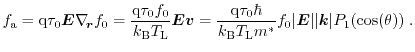
The quantum mechanical current density is defined as [45]
with
 as the transposed conjugate complex form of
 .
.
However, the situation is more complex in real semiconductors. Here, the band
structure together with the electrostatic energy
 as
described in Section 1.1.1 plays an important role.
Fig. 1.2 shows a cross-section of a typical p-type MOSFET
device under inversion [46]. Due to the applied gate voltage,
the conduction band forms a potential well. Therefore, the so called quantum
confinement occurs, if the carriers in bound states cannot propagate to
infinity. Hence, the potential well forms a boundary condition.
as
described in Section 1.1.1 plays an important role.
Fig. 1.2 shows a cross-section of a typical p-type MOSFET
device under inversion [46]. Due to the applied gate voltage,
the conduction band forms a potential well. Therefore, the so called quantum
confinement occurs, if the carriers in bound states cannot propagate to
infinity. Hence, the potential well forms a boundary condition.
Figure 1.2:
Quantum confinement in a MOSFET structure
|
|
Within this well, discrete energy levels, the so called energy subbands occur,
which will be discussed in Section 1.2. Due to the quantum
confinement, the carriers cannot move in the direction perpendicular to the
interface, and therefore carrier transport is just in the two-dimensional plane
parallel to the oxide [47]. For increasing lateral fields the
carriers can go beyond the last occupied subband and become a three-dimensional
carrier gas. This can be explained as follows:
Assuming a triangular potential, which is an analytical approximation for the
inversion layer, the wavefunctions are the well known Airy functions,
whereas the energy eigenvalues can be expressed as [48]
with  as a constant and
  is the number of the
th subband. The difference
between the
th and the
is the number of the
th subband. The difference
between the
th and the  th subband can be written as
This difference as a function of the number of subbands is visualized
in Fig. 1.3. For increasing number of subbands the energy gap
decreases. Furthermore for an infinite number of energy eigenvalues this gap
converges to zero. Thus, the subband system is transformed into a bulk system
for an infinite number of subbands.
Figure 1.3:
For increasing subbands the difference between the energy eigenvalues
decreases and converge to zero for an infinite number of
energy-eigenstates. In this limit the subband system becomes a bulk system.
|
|
In order to correctly describe energy eigenvalues and wavefunctions in a
device, the Schrödinger
equation has to be solved self-consistently with Poisson's
equation [49,2]. The starting point for solving the
system is a potential distribution, which leads to charge neutrality. Inserting
the potential into the Schrödinger equation, one obtains the initial energy
eigenvalues
 and wavefunctions
for the quantum
mechanical carrier concentration defined as
and wavefunctions
for the quantum
mechanical carrier concentration defined as
Here,
 denotes the effective density of states
 |
(1.14) |
with
 as the degeneracy of the system.
The next step is a recalculation of the potential by Poisson's equation
followed by new wavefunctions and energy eigenvalues. These steps are performed
in a loop until the update is below a certain limit, thus convergency is
reached.
Figure 1.4:
Conduction band and the first two wavefunctions of a thin film SOI
MOSFET for different gate voltages. For increasing gate
voltages the wavefunctions are shifted towards the interface.
|
|
Results from a Schrödinger-Poisson solver are presented
in Fig. 1.4 [50].
Here, the first energy subband together with two wavefunctions for different
gate voltages as a function of the channel thickness are highlighted. Due to
the shift of the wavefunctions to the oxide for high gate voltages, the
carriers are strongly localized. Therefore, the impact of interface effects as
surface roughness scattering for high gate voltages is very strong.
1.1.3 Boltzmann's Transport Equation
The basic equation of macroscopic transport description, the BTE, is
derived using fundamental principles of statistical mechanics. The first part
concerns the discussion of the solution of the BTE, whereas the second
part is devoted to its derivation.
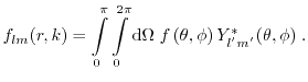
1.1.3.1 The Distribution Function
The carrier distribution function
 is the solution of the
BTE [1].
is the probability of the number of particles
having approximately the momentum
is the solution of the
BTE [1].
is the probability of the number of particles
having approximately the momentum
 near the position
 in phase
space and time
in phase
space and time
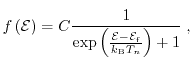
 . Taking Pauli's exclusion principle into account, the
thermal equilibrium distribution function is the Fermi-Dirac function (equilibrium
solution of the BTE)
. Taking Pauli's exclusion principle into account, the
thermal equilibrium distribution function is the Fermi-Dirac function (equilibrium
solution of the BTE)
 |
(1.15) |
with  as a normalization factor, whereas
 is the
Fermi energy.
Fig. 1.5 shows the Fermi-Dirac function for 0
is the
Fermi energy.
Fig. 1.5 shows the Fermi-Dirac function for 0
 , 300
, and
500
. For 0
, the Fermi-Dirac function can be written as a step function
, 300
, and
500
. For 0
, the Fermi-Dirac function can be written as a step function
 . Hence, all states are fully occupied below
. For increasing temperatures, states above
can be occupied, which results
in a smoother transition. The energy range of the transition region is
. Hence, all states are fully occupied below
. For increasing temperatures, states above
can be occupied, which results
in a smoother transition. The energy range of the transition region is
 (see Fig. 1.5).
Figure 1.5:
Fermi-Dirac distribution function for
 ,
,
 ,
,
 , and the limit
 is demonstrated. In this limit, the Fermi-Dirac function can be approximated
by a Maxwell distribution function.
is demonstrated. In this limit, the Fermi-Dirac function can be approximated
by a Maxwell distribution function.
|
|
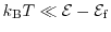
If the relation
is fulfilled, the Fermi-Dirac distribution function can be approximated by the Maxwell distribution function
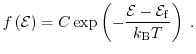 |
(1.17) |
The Maxwell distribution function neglects Pauli's exclusion principle.
Therefore, the validity is limited to lowly doped, non-degenerate semiconductors.
An important approximation used in the derivation of macroscopic transport
models (see Section 1.4.3) is the diffusion approximation, which will
be discussed here.
Every distribution function can be split into a symmetric
 and an
anti-symmetric
and an
anti-symmetric
 part as
 |
(1.18) |
Within the diffusion approximation it is assumed that the displacement of the distribution
function is small, which means that
is much smaller than
[51]. One of the consequences of this approximation is
that only the diagonal elements of the average tensorial product of for
instance the momentum
contribute, while the off diagonal elements can be neglected, due to symmetry reasons.
The average operation used in equation (1.19) is the normalized
statistical average and will be described in Section 1.4.3.
In general, the average energy of the carriers can
be decomposed into
where
 is the kinetic energy part and
 is the thermal energy part of the average
carrier energy. Within the diffusion approximation the kinetic part of
equation (1.20) is neglected.
is the thermal energy part of the average
carrier energy. Within the diffusion approximation the kinetic part of
equation (1.20) is neglected.
1.1.3.3 Derivation of Boltzmann's Transport Equation
The Boltzmann's transport equation is derived from a fundamental principle
of classical statistical mechanics, the Liouville
theorem [52,53]. The proposition asserts that
the many particle distribution function
 along phase-space trajectories
 is constant for all times
  [54]. With the
total derivation of the many particle distribution function, the Liouville
theorem can be expressed as
[54]. With the
total derivation of the many particle distribution function, the Liouville
theorem can be expressed as
Due to the Hamilton equations
and the Poisson bracket defined as
 |
(1.23) |
the Liouville equation (1.21) can be written in a very compact
form as
Equation (1.24) has to be solved in the
 space, where
 is the number of
particles and
is the number of
particles and
 is a dimension factor. The initial condition is
defined as
is a dimension factor. The initial condition is
defined as
is naturally very large and therefore the solution of
(1.24) is very expensive.
To derive a lower-dimensional equation, Vlasov introduced a single particle
Liouville equation with a force
 [55]
[55]
 |
(1.26) |
Many-particle physics is taken into account in Vlasov's equation through the
force
and the assumption that the probability to occupy a state
along phase trajectories is constant. The force can be split into an external
and a long-range interaction force. However, the main disadvantage of
Vlasov's equation is that it does not provide a description of strong
short-range forces such as scattering of particles with other particles or with
the crystal. So, an extended Vlasov equation must be formulated to treat
these important transport effects. Introducing the scattering operator
 , the balance equation for the distribution
function must fulfill the conservation equation
, the balance equation for the distribution
function must fulfill the conservation equation
Hence, scattering allows particles to jump from one trajectory to another
(see Fig. 1.6).
Figure 1.6:
Scattering event from one trajectory to another in phase
space. Scattering events, which are assumed to happen instantly, change the carrier's
momentum, while the position is not affected (after [1]).
|
|
With the full derivative of the distribution function and
equation (1.22), the Boltzmann's transport
equation (1.27) can be finally expressed in the common form as
Equation (1.28) is a semi-classical equation
containing Newton mechanics on the left side, and the quantum mechanical
scattering operator on the right side. Still, it remains to formulate an
expression for the scattering operator
 . There exist many strategies
for modeling the scattering operator [16,4]. To develop solution strategies
for the semi-classical differential equation, it is important to discuss the
underlying limitations and assumptions of the BTE:
. There exist many strategies
for modeling the scattering operator [16,4]. To develop solution strategies
for the semi-classical differential equation, it is important to discuss the
underlying limitations and assumptions of the BTE:
 The original many particle problem is replaced by a one particle problem with an
appropriate potential. Due to the Hartree-Fock approximation
[56], the contribution of the surrounding electrons to this
potential is approximated by a charge density. Furthermore, the short
range electron-electron interaction cannot be described. However,
the potential of the surrounding carriers is treated by the electric field
self-consistently.
The original many particle problem is replaced by a one particle problem with an
appropriate potential. Due to the Hartree-Fock approximation
[56], the contribution of the surrounding electrons to this
potential is approximated by a charge density. Furthermore, the short
range electron-electron interaction cannot be described. However,
the potential of the surrounding carriers is treated by the electric field
self-consistently.
The distribution function
 is a classical concept due to the negligence
of Heisenberg's uncertainty principle. The distribution function specifies
both the position and the momentum at the same time.
is a classical concept due to the negligence
of Heisenberg's uncertainty principle. The distribution function specifies
both the position and the momentum at the same time.
Due to the uncertainty principle, the mean free path of the particles
must be longer than the mean De Broglie wavelength.
Semi-classical treatment of carriers as particles obey Newton's
law.
Collisions are assumed to be binary and to be instantaneous in time and local in
space.
It is important to have these limitations in mind, while deriving transport
models based on the BTE. However, as has been reported in many
publications [57,58,59,60],
models based on the BTE give good results in the scattering dominated
regime. Thus, it is a good starting point for simpler macroscopic transport
models such as the drift-diffusion, the hydrodynamic, or even higher-order
models.
1.2 Band Structure
The focus of this section is put on the band structure of bulk silicon and the
occurrence of subbands. Furthermore, results are presented, which show the
influence of the band structure on the transport properties.
Carriers in a crystal are moving in a periodic potential energy
 .
Due to this periodic potential, the solution of the time-independent
.
Due to this periodic potential, the solution of the time-independent
 equation
are the so called Bloch waves expressed as [61,62]
The boundary condition
 |
(1.31) |
must hold, with  as the lattice constant.
Inserting the Bloch waves (1.30) into
equation (1.29) the Schrödinger equation can be written
as
as the lattice constant.
Inserting the Bloch waves (1.30) into
equation (1.29) the Schrödinger equation can be written
as
The so called
 method gives approximate solutions
to (1.32) [63,64]. Several other methods
such as pseudo-potential calculations [65,66], tight
binding [67], Hartree-Fock [68], and density
functional theory [69] have been proposed to calculate the full
band structure within the first Brillouin zone.
method gives approximate solutions
to (1.32) [63,64]. Several other methods
such as pseudo-potential calculations [65,66], tight
binding [67], Hartree-Fock [68], and density
functional theory [69] have been proposed to calculate the full
band structure within the first Brillouin zone.
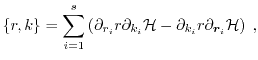
If the band structure is already given,
 can be expanded
around the band edge minimum into a Taylor series as
can be expanded
around the band edge minimum into a Taylor series as
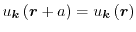
Here the Taylor series is truncated after the second derivative. The energy
minimum is assumed at
 following that the term with the first derivative
can be neglected. Thus the energy can be expressed as
following that the term with the first derivative
can be neglected. Thus the energy can be expressed as
With a comparison between equation (1.34) and the energy dispersion relation
the inverse effective mass tensor can be written as
 |
(1.36) |
So electrons in a crystal can be assumed as free particles with a direction
dependent mass. For silicon, the effective mass yields [44]
 |
(1.37) |
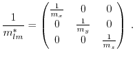
Furthermore, the effective mass of cubic semiconductors depends on the
crystallographic orientation of the applied field. With the so called
longitudinal mass or heavy hole mass
 and the transversal mass or light
hole mass
and the transversal mass or light
hole mass
 , the energy dispersion relation can be defined as
Equation (1.38) is a band with ellipsoidal constant energy surfaces as
depicted in Fig. 1.7.
Figure 1.7:
Energy ellipsoids of the first conduction band within the first
Brillouin zone of silicon (after [2]).
|
|
These are the six valleys of the first conduction band of silicon.
Due to the truncation after the second-order derivative of the Taylor
series, the effective mass approximation is only valid for low fields. Thus,
the assumption of parabolic bands is not valid anymore for high fields. With
the introduction of a non-parabolicity factor
, as proposed
by Kane [70,47,71], the parabolic dispersion
relation (1.35) can be rewritten into a first order correction
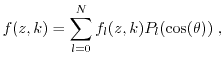
A direct consequence of the band structure is the density of states, which
describes the energetical density of electronic states per
volume [1]
 |
(1.40) |
In the parabolic band approximation the density of states for one, two, and
three-dimensions reads as
For the non-parabolic dispersion relation (1.39) the density of states can
be formed as
Note that in the two-dimensional case for non-parabolic bands the density of
states is energy dependent, whereas for a parabolic band structure the density
of states is energy independent. Equation (1.39) is valid up to energies
of
 [1]. Therefore, to model high-field
transport, a more sophisticated description has to be found. One possibility,
which is used in this work, is to calculate non-parabolic factors as a post
processing step from Monte Carlo simulations. This procedure will be explained
in Section 1.4.3.
In Section 1.1.2, an introduction of the Schrödinger-Poisson
loop including inversion layer effects has been given. In real devices within
the crystallographic orientation
[1]. Therefore, to model high-field
transport, a more sophisticated description has to be found. One possibility,
which is used in this work, is to calculate non-parabolic factors as a post
processing step from Monte Carlo simulations. This procedure will be explained
in Section 1.4.3.
In Section 1.1.2, an introduction of the Schrödinger-Poisson
loop including inversion layer effects has been given. In real devices within
the crystallographic orientation ![$ [001]$](img187.png) , the valley, which has its
longitudinal mass perpendicular to the interface surface, gives rise to a
ladder of subbands, the so called unprimed valley, whereas the other valleys
give rise to an other, higher lying ladder in the primed and double primed
valleys [72]. It has been pointed out in [47] that by
inserting the mass tensor (1.37) into the Schrödinger equation, the
energy dispersion relation of the orientation
can be described as
, the valley, which has its
longitudinal mass perpendicular to the interface surface, gives rise to a
ladder of subbands, the so called unprimed valley, whereas the other valleys
give rise to an other, higher lying ladder in the primed and double primed
valleys [72]. It has been pointed out in [47] that by
inserting the mass tensor (1.37) into the Schrödinger equation, the
energy dispersion relation of the orientation
can be described as
with
 as the quantization direction.
 is the bottom energy of
the ith subband. Equation (1.44) represents constant
energy-parabolas above
, the so called subband ladders. Inserting the
corresponding longitudinal mass or the transversal mass of the valley into
equation (1.44), one yields the subband ladders of the unprimed,
primed, and double primed valleys, respectively.
is the bottom energy of
the ith subband. Equation (1.44) represents constant
energy-parabolas above
, the so called subband ladders. Inserting the
corresponding longitudinal mass or the transversal mass of the valley into
equation (1.44), one yields the subband ladders of the unprimed,
primed, and double primed valleys, respectively.
Fig. 1.8 shows the subband ladders of the unprimed and primed
valleys. Since the double primed and the primed valleys have the same energy
subband values, due to the identical quantization mass, only the primed ladders
are visualized. Due to the fact that the energy is inversely proportional to
the quantization mass the energies of the primed ladders are higher than the
ones from the unprimed ladders [73]. The quantization mass of the
unprimed and primed valleys are
 and
and
 , respectively. The
subband occupations within high fields have got a strong influence on the
carrier transport properties as demonstrated in Fig. 1.9
and Fig. 1.10
, respectively. The
subband occupations within high fields have got a strong influence on the
carrier transport properties as demonstrated in Fig. 1.9
and Fig. 1.10
In Fig. 1.9, the subband occupation as a function of the
driving field of an example device is presented. Carriers gain kinetic energy,
which results in a re-occupation of higher subband ladders. Due to this
re-occupation for high fields, the carrier wavefunctions are shifted within the
inversion layer, which inherently affects the overlap integral of the
scattering operator. Furthermore, the subband ladder reconfiguration leads to a
variation of the spatial distribution function of the electrons, which itself
has an impact on the shape of the potential well that forms the inversion
channel.
Figure 1.8:
Unprimed and primed subband ladders
|
|
Figure 1.9:
Populations of the first two subbands in the unprimed, primed, and
double primed valleys versus lateral field in a UTB SOI MOSFET test
device. Relative occupations are shifted to higher subbands in each valley for higher fields.
|
|
The carrier velocity of the first and the second subband is displayed
in Fig. 1.10.
Figure 1.10:
Velocities of the first and second subband of the unprimed, primed,
and double primed valleys as well as the average total velocity versus lateral electric field.
|
|
Due to different conduction masses in transport direction of each valley as
well as a strong occupation of the primed valley in the high field regime (see
Fig. 1.9), the total velocity is lower than in the unprimed
and double primed valley [50]. A detailed discussion about
subbands is given in [47].
An introduction of the most common quantum transport models, namely the
non-equilibrium Green's function method, the Wigner Monte Carlo technique, and
quantum macroscopic models is given, followed by a discussion of quantum
correction models suitable for semi-classical models.
1.3.1 Non-Equilibrium Green's Function Method
The non-equilibrium Green's function (NEGF) is a very powerful technique to
describe open systems fully quantum mechanically.
This method has been extensively used in modeling nanoscale transistors and is
an efficient way of computing quantum effects in devices as subband
quantization, tunneling, and quantum reflections. It is exact in the ballistic
regime. Recently scattering processes have been included, which, however,
requires considerable computational power. Furthermore NEGF allows to study
the time evolution of a many-particle open quantum system. The many-particle
information about the system is set into self-energies, which are parts of the
equations of motion for the Green's functions. Green's functions can be
calculated from perturbation theory [74]. The NEGF technique
is a sophisticated method to determine the properties of a many-particle system
both in thermodynamic equilibrium as well as in non-equilibrium situations. In
the sequel, a description of the quantum transport method for the single
particle model is given. For open systems with a coupling to a reservoir,
the Hamiltonian, which describes the quantum system, can be expressed
as [31,75]
 |
(1.45) |
with
 and
and
 as the Hamilton operators of the contact and the
channel respectively, and
as the Hamilton operators of the contact and the
channel respectively, and  denoting the coupling matrix. Hence, the Schrödinger equation of the
channel-contact system can be written as [76]
denoting the coupling matrix. Hence, the Schrödinger equation of the
channel-contact system can be written as [76]
Here,
 and
and
 are the wavefunctions of the channel and
the contact, respectively.
The Green's function equation is defined as
are the wavefunctions of the channel and
the contact, respectively.
The Green's function equation is defined as
 |
(1.47) |
and therefore the corresponding Green's function to (1.46) can be
expressed as [31]
where
 and
and
 describe the coupling between device and
the reservoir, whereas
describe the coupling between device and
the reservoir, whereas
 is the Green's function of the reservoir itself.
The retarded Green's function
is the Green's function of the reservoir itself.
The retarded Green's function  can be written as
 is the energy dependent self-energy and describes the interaction
between the device and the
reservoir [77,78,79]. Thus, the advantage of the
self-energy is that it reduces the Green's function of the reservoir to the
dimension of the device Hamiltonian. The self-energy can be obtained as
is the energy dependent self-energy and describes the interaction
between the device and the
reservoir [77,78,79]. Thus, the advantage of the
self-energy is that it reduces the Green's function of the reservoir to the
dimension of the device Hamiltonian. The self-energy can be obtained as
 |
(1.50) |
and is usually determined iteratively. The spectral function  can
be written as
can
be written as
 is the matrix form of the density of
states
is the matrix form of the density of
states
 . Finally, the density matrix can be expressed as
 |
(1.52) |
which provides the charge distribution in the channel.
 is the Fermi
distribution function as explained in Section 1.1.3 and
is
the Fermi energy.
is the Fermi
distribution function as explained in Section 1.1.3 and
is
the Fermi energy.
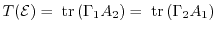
Assuming that the device is being connected to two
contacts with different Fermi energies and hence also different Fermi
functions, the current in the ballistic regime can be obtained
as [78]
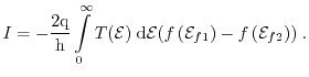 |
(1.53) |
 is the transmission coefficient indicating the probability, that an
electron with the energy
is the transmission coefficient indicating the probability, that an
electron with the energy
 can travel from the source to the drain and is
defined as
can travel from the source to the drain and is
defined as
 |
(1.54) |
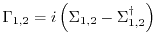
with
 |
(1.55) |
as the coupling of the channel to the reservoir.
The MC technique is a well established and accurate numerical method to
solve the BTE. Due to the similarities between the Wigner equation
written as [80,81]
and the BTE (see equation (1.28)), it is tempting to
solve the Wigner equation with the MC
technique [82,83,33] as well.
 denotes an external Wigner potential. The Wigner function
 can be
derived from the density matrix expressed by the Liouville von Neumann equation using
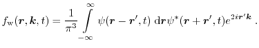
the Wigner-Weyl transformation [84]. With the Fourier
transformation of the product of wavefunctions at two
points [85], the Wigner function can be expressed as
can be
derived from the density matrix expressed by the Liouville von Neumann equation using
the Wigner-Weyl transformation [84]. With the Fourier
transformation of the product of wavefunctions at two
points [85], the Wigner function can be expressed as
 |
(1.57) |
The Wigner function is a quantum mechanical description in phase-space,
which is, however no longer positive definite. Hence, it cannot be regarded as
a distribution function directly, but observables need to be derived from it.
In the literature this is known as the negative-sign
problem [86,87].
An important feature of this so
called phase-space approach is the ability of expressing quantum mechanical
expectation values in the same way as it is done in classical statistical
mechanics.
Furthermore, the Wigner equation can be used as a base for
quantum macroscopic transport models as the quantum drift-diffusion or the
quantum hydrodynamic model using the method of moments.
1.3.3 Quantum Macroscopic Models
Quantum macroscopic models can be derived from a fluid dynamical view using
the Madelung transformation for the wave function
defined
as [39]
The Madelung transformation states that the wave function can be decomposed
in its amplitude
 and phase
 , whereby the amplitude is
defined as the square root of the particle density.
, whereby the amplitude is
defined as the square root of the particle density.
 is referred here
to the complex number
is referred here
to the complex number  , whereas
 denotes the carrier mass.
Since the electron density of a single state is defined
as [39]
denotes the carrier mass.
Since the electron density of a single state is defined
as [39]
and the density is by definition positive, the Madelung transformation makes
only sense as long as
 is valid [53].
Quantum macroscopic models can be derived from the Wigner equation as well
using the method of moments. Since macroscopic transport models based on
the BTE are derived using the method of moments (see Section 1.4.1),
only the derivation of quantum macroscopic models using the Madelung
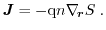
transformation is pointed out here. Inserting equation (1.58) into
equation (1.11), the current density
 can be written
as
can be written
as
 |
(1.60) |
The phase
of equation (1.58) can be interpreted as a velocity
potential. Inserting equation (1.58) into the Schrödinger
equation (1.7) yields
Dividing equation (1.61) with
 leads to
 |
(1.61) |
 |
|
With the imaginary part, one can obtain the particle conservation equation as
The real part yields
With the gradient and a multiplication of (1.64) with
 , one
obtains the quantum conservation equation of the current
, one
obtains the quantum conservation equation of the current
Equations (1.63) and
(1.65) are referred to as the quantum
hydrodynamic equations [39]. With ``
 '',
the quantum conservation equation (1.65) turns
into the classical current conservation equation. The advantage of this method
is that in two or three space dimensions fluid-dynamical models are numerical
cheaper compared to the Schrödinger equation. Furthermore, boundary conditions
can be more easily applied compared to the Schrödinger
formulation. However, the dispersive character of the quantum hydrodynamic
transport system implies that the solution may develop high frequency
oscillations, which are localized in regions not a priori known. Therefore, the
numerical simulations with quantum hydrodynamic models require an extremely
high number of grid points, which leads to unnecessarily time consuming
computations [88].
'',
the quantum conservation equation (1.65) turns
into the classical current conservation equation. The advantage of this method
is that in two or three space dimensions fluid-dynamical models are numerical
cheaper compared to the Schrödinger equation. Furthermore, boundary conditions
can be more easily applied compared to the Schrödinger
formulation. However, the dispersive character of the quantum hydrodynamic
transport system implies that the solution may develop high frequency
oscillations, which are localized in regions not a priori known. Therefore, the
numerical simulations with quantum hydrodynamic models require an extremely
high number of grid points, which leads to unnecessarily time consuming
computations [88].
1.3.4 Quantum Correction Models
Since transport parameters as for instance the carrier mobility of modern
semiconductor devices are strongly influenced by quantum mechanical effects, it
is essential to take quantum correction models within classical simulations
into account. Several quantum correction models based on different approaches
have been proposed, which influence the electrostatics of the system.
The quantum correction model modified local density approximation (MLDA) [89] is based
on a local correction of the effective density of states
 near the gate oxide
as
near the gate oxide
as
 is here the classical effective density of states with
 as a
fitting parameter.
is the distance from the interface,
as a
fitting parameter.
is the distance from the interface,
 is
the tunneling distance, and
is
the tunneling distance, and
 denotes the thermal wavelength. The
correction term of equation (1.66) can be calculated from the
quantum mechanical expression of the particle density as stated
in [90]. The advantage of the MLDA procedure is that no
solution variable is used in the correction term. Therefore, the model can be
implemented as a preprocessing step and has only a minor impact on the overall
CPU time [91]. However, this approach is based on the
field-free Schrödinger equation. The method loses its validity for
high-fields. An improved MLDA technique has been suggested
in [92,93]. A heuristic wavelength parameter has been
introduced as
denotes the thermal wavelength. The
correction term of equation (1.66) can be calculated from the
quantum mechanical expression of the particle density as stated
in [90]. The advantage of the MLDA procedure is that no
solution variable is used in the correction term. Therefore, the model can be
implemented as a preprocessing step and has only a minor impact on the overall
CPU time [91]. However, this approach is based on the
field-free Schrödinger equation. The method loses its validity for
high-fields. An improved MLDA technique has been suggested
in [92,93]. A heuristic wavelength parameter has been
introduced as
 |
(1.67) |
where
 is defined as the net doping
 with
with
 as a fit factor. As pointed out in [92], the
improved MLDA can now cover the important case of high fields
perpendicular to the interface. The fit parameters have been matched with the
results of a self-consistent Schrödinger-Poisson solver. The model is
calibrated for bulk MOSFET structures. However, the MLDA method is only
valid for devices with one oxide. Therefore, a characterization of quantization
in DG MOSFETs is not possible.
as a fit factor. As pointed out in [92], the
improved MLDA can now cover the important case of high fields
perpendicular to the interface. The fit parameters have been matched with the
results of a self-consistent Schrödinger-Poisson solver. The model is
calibrated for bulk MOSFET structures. However, the MLDA method is only
valid for devices with one oxide. Therefore, a characterization of quantization
in DG MOSFETs is not possible.
A quantum correction technique to cover such devices is presented
in [94]. The idea behind this model is as follows: The strong
quantization perpendicular to the interface can be well approximated with an
infinite square well potential. The eigenstates within the quantization region
are estimated using an analytical approach. This assumption allows to determine
a quantum correction potential which modifies the band edge to reproduce the
quantum mechanical carrier concentration.
In [95], the correction is carried out by a better
modeling of the conduction band edge as
 with with  |
(1.68) |
 is the classical band edge energy, the correction
 is a
function of the distance to the interface, and
is a
function of the distance to the interface, and
 is the
electric field perpendicular to the interface. The value of the
proportionality factor can be determined from the shift of the long-channel
threshold voltage as explained in [95].
is the
electric field perpendicular to the interface. The value of the
proportionality factor can be determined from the shift of the long-channel
threshold voltage as explained in [95].
Fig. 1.11 shows the electron concentration calculated for a
single gate SOI MOSFET classically, quantum mechanically, and with the quantum
correction models MLDA, the model after [95], and
the improved modified local density approximation (IMLDA)[92]. A gate voltage
of
 has been applied, and the quantum electron concentration
has been calculated using a Schrödinger-Poisson
solver [2]. As can be observed, the electron concentration
obtained from the IMLDA model fit the quantum mechanical simulation quite
well compared to the other approaches. Therefore, the IMLDA model is used in
this work to cover quantum effects in the classical device simulations.
has been applied, and the quantum electron concentration
has been calculated using a Schrödinger-Poisson
solver [2]. As can be observed, the electron concentration
obtained from the IMLDA model fit the quantum mechanical simulation quite
well compared to the other approaches. Therefore, the IMLDA model is used in
this work to cover quantum effects in the classical device simulations.
Figure 1.11:
The electron concentration of a single gate SOI MOSFET has been
calculated classically, quantum-mechanically, together
with the quantum correction models MLDA, Van Dort, and the
improved MLDA (after [3]).
|
|
The main focus of this work is set on macroscopic transport models based on
the BTE. First, the method to derive higher-order macroscopic models is
described followed by a detailed derivation. Since the models must be
benchmarked to other solution techniques of
the BTE [96,97], a short introduction of
the Monte Carlo method and the Spherical Harmonics Expansion approach is presented.
1.4.1 Method of Moments
On an engineering level, a very efficient way to find approximate solutions of
the BTE is the method of moments. In order to formulate a set of balance
and flux equations coupled with Poisson's equation, one has to multiply
the BTE with a set of weight functions and integrate over
 -space.
An arbitrary number of equations can be derived, each containing information
from the next-higher equation. Hence, there exists more moments than
equations. Therefore, one has to truncate this equation hierarchy in order to
get a fully defined equation-system. The assumption to close the system and to
express the highest moment with the lower moments is called closure
relation. The closure relation estimates the information of the higher-order
moments and thus determines the accuracy of the system. For instance, in the
case of the drift-diffusion model, the electrons are assumed to be in thermal
equilibrium (
 ) with the lattice [1].
There exist several theoretical approaches to cover the closure
problem [98], like the maximum entropy
principle [99,100,101] in the sense of extended
thermodynamics.
) with the lattice [1].
There exist several theoretical approaches to cover the closure
problem [98], like the maximum entropy
principle [99,100,101] in the sense of extended
thermodynamics.
The idea of the maximum entropy principle is that a large number of collisions
is necessary to relax the carrier energies to their equilibrium, while the
momentum, heat flow, and anisotropic stresses relax within a shorter
time. Therefore, an intermediate state arises, where the fluid is in its own
thermal equilibrium. This can be called partial thermal equilibrium. All transport parameters are
zero except for the carrier temperature
 . Another important assumption is
that the entropy density and the entropy flux do not depend on the relative
velocity of the electron gas. With the partial thermal equilibrium, closure relations can be found
which are exactly those obtained with a shifted Maxwellian. A
heated Maxwellian is used here as a closure for the hydrodynamic transport
model and by the introduction of the kurtosis, the six moments model will be
closed. A detailed description is given in the sequel.
. Another important assumption is
that the entropy density and the entropy flux do not depend on the relative
velocity of the electron gas. With the partial thermal equilibrium, closure relations can be found
which are exactly those obtained with a shifted Maxwellian. A
heated Maxwellian is used here as a closure for the hydrodynamic transport
model and by the introduction of the kurtosis, the six moments model will be
closed. A detailed description is given in the sequel.
To get physically reasonable equations, the weight functions are chosen as the
powers of increasing orders of the momentum. The moments in one, two, and three
dimensions, respectively, are defined as
 |
(1.69) |
 denotes the macroscopic values together with the microscopic
counterpart
denotes the macroscopic values together with the microscopic
counterpart
 , where
 is the time dependent distribution
function in the six-dimensional phase space.
is the time dependent distribution
function in the six-dimensional phase space.
 is linked to the one, two,
and three-dimensional electron gas (
is linked to the one, two,
and three-dimensional electron gas (
 ,
,
 , or
, or
 ), whereas
represents the carrier density.
), whereas
represents the carrier density.
For the sake of clarity, during the derivation of macroscopic transport models
the dimension indices are neglected. Multiplying the BTE with the even
scalar-valued weights
 and integrating over
-space
and integrating over
-space
yields the general conservation equations. In the following derivations, the
distribution
, the group velocity
 , and the generalized force
 are denoted as
,
are denoted as
,
 , and
, and
 .
.
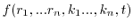
The first term on the left side of equation (1.70) leads to
whereas the second term yields
and the third term
Using Gauss'theorem and assuming that all surface integrals over
the border of the Brioullin-Zone are equal to zero [102], the first term
on the right side of equation (1.73)
vanishes. Inserting
 and
and
 with the Hamilton function
given as
with the Hamilton function
given as
with
 for electrons and
 for holes, into equation (1.72)
and (1.73) respectively, leads to the BTE expressed by the
averages of the even scalar-valued moment
for holes, into equation (1.72)
and (1.73) respectively, leads to the BTE expressed by the
averages of the even scalar-valued moment
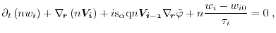
Finally, the equation reads
Furthermore, the BTE for the odd vector-valued moments can be transformed
analogously
Equations (1.76) and (1.77) are the
starting points for the derivations of the conservation equations and fluxes of macroscopic transport models.
In order to get an analytical expression for the right hand side of
equations (1.76) and (1.77)
several approaches have been suggested in [103,16]. In this work, the macroscopic relaxation time
approximation after Bløtekjær [104] is used to approximate the scattering
operator of the BTE
 is the macroscopic relaxation time for the weight
function
is the macroscopic relaxation time for the weight
function
 .
.
 is the average weight function in
equilibrium. Since the relaxation time
depends on the
distribution function, equation (1.78) is not an approximation.
With
is the average weight function in
equilibrium. Since the relaxation time
depends on the
distribution function, equation (1.78) is not an approximation.
With
equation (1.78) turns into the macroscopic relaxation time
approximation. Therefore, the relaxation times depends only on the moments of
the distribution function.
For the odd moments, the approximation yields
 |
(1.80) |
and for the even moments one obtains
 |
(1.81) |
The subscript odd and even is linked to whether the moment is even or odd.
1.4.3 Macroscopic Transport Models
A hierarchy of macroscopic transport models based on the equations
(1.76) and (1.77) can be derived using the
method of moments described above [105].
The first three even scalar valued moments are defined as the powers of the energy

and the first three odd vector valued moments are defined as
In order to obtain the particle balance equation and the current equation, one
has to insert the zeroth moment
 and the first moment
 into
equation (1.76) and (1.77), respectively.
While in the particle balance equation the particle current remains as an unknown variable, the particle
current equation comprises the average kinetic energy. With a heated
Maxwellian and the diffusion approximation the powers of the average energy
assuming a parabolic band structure can be expressed by the carrier temperature as
into
equation (1.76) and (1.77), respectively.
While in the particle balance equation the particle current remains as an unknown variable, the particle
current equation comprises the average kinetic energy. With a heated
Maxwellian and the diffusion approximation the powers of the average energy
assuming a parabolic band structure can be expressed by the carrier temperature as
for the one, two, and three-dimensional electron gas, respectively. For instance, the
average energy ( ) for the 3D case can be written as
The drift-diffusion model is closed by the assumption of local thermal equilibrium, thus the carrier
temperatures are set to the lattice temperature. The energy balance equation is
introduced taking the second moment
into account, where the
energy flux remains as an unknown term. The third moment
 describes exactly this energy
flux. The transport model considering these first four moment
equations is called the hydrodynamic transport model [4].
By considering additional moments
describes exactly this energy
flux. The transport model considering these first four moment
equations is called the hydrodynamic transport model [4].
By considering additional moments
 and
and
 , leads to the
second-order temperature balance equation and to the second-order temperature
flux. The so called six moments model is closed by introducing the kurtosis
, leads to the
second-order temperature balance equation and to the second-order temperature
flux. The so called six moments model is closed by introducing the kurtosis
 describing the deviation of the
current distribution function from the Maxwell distribution
function [106].
describing the deviation of the
current distribution function from the Maxwell distribution
function [106].
The assumptions made during the derivation of the transport model are specified
as follow:
- Non-parabolic band structure
- Product ansatz for the kinetic energy
- Isotropic band structure
- Tensor valued parameters are approximated by their traces
- Macroscopic relaxation time approximation
- Diffusion approximation
- Homogeneous materials
Furthermore, the averages of the microscopic quantities are defined as
 and
and
 In the case of the
six moments model,
is defined in the range
In the case of the
six moments model,
is defined in the range
![$ i{\;}\in[0,2]$](img315.png) .
A detailed derivation and discussion of these models follows in the next section.
An important objective here is to point out the model limitations.
.
A detailed derivation and discussion of these models follows in the next section.
An important objective here is to point out the model limitations.
1.4.3.1 Drift-Diffusion Transport Model
Inserting the zeroth moment
into equation (1.76) yields the particle balance
equation
Since
depends neither on
or
 , one can omit the
third, the fourth, and the fifth term of equation (1.86) to obtain
, one can omit the
third, the fourth, and the fifth term of equation (1.86) to obtain
Inserting the first moment
into equation (1.77),
the particle flux is obtained. The time derivation terms of the fluxes are
neglected, since the relaxation time is in the order of picoseconds, which ensures
quasi-stationary behavior even for today's fastest signals [107,20].
where
 is the momentum relaxation time.
Due to the assumption of an isotropic band structure and in the diffusion
limit, the non-diagonal elements of the tensors of
equation (1.88) vanish. Hence, the tensor of the first part
(1)
of
equation (1.88) can be approximated as the trace divided
by the dimension factors of the system. Multiplying
(1)
with tensorial
non-parabolicity factors
is the momentum relaxation time.
Due to the assumption of an isotropic band structure and in the diffusion
limit, the non-diagonal elements of the tensors of
equation (1.88) vanish. Hence, the tensor of the first part
(1)
of
equation (1.88) can be approximated as the trace divided
by the dimension factors of the system. Multiplying
(1)
with tensorial
non-parabolicity factors
 , one obtains
 |
(1.89) |
with
 as a dimension factor.
can be calculated considering the dimension of the system and the
prefactors of the average energy assuming a parabolic bandstructure and a Maxwell distribution function.
For instance, in the case of the three-dimensional electron gas the value of
can be
derived as
as a dimension factor.
can be calculated considering the dimension of the system and the
prefactors of the average energy assuming a parabolic bandstructure and a Maxwell distribution function.
For instance, in the case of the three-dimensional electron gas the value of
can be
derived as
 |
(1.90) |
is equal to  . The average energy has been considered according
to equation (1.85).
For the one and two-dimensional electron gas the values are
. The average energy has been considered according
to equation (1.85).
For the one and two-dimensional electron gas the values are
 and
and
 ,
respectively. In the sequel, the non-parabolic factors will be shown using
Subband Monte Carlo (SMC) data for the two-dimensional electron gas.
,
respectively. In the sequel, the non-parabolic factors will be shown using
Subband Monte Carlo (SMC) data for the two-dimensional electron gas.
 represents
the effective masses for electrons and holes respectively.
represents
the effective masses for electrons and holes respectively.
Based on the second assumption that the kinetic energy can be expressed using a
product ansatz
 |
(1.91) |
term
(2)
and
(3)
of (1.88) vanish. The
fourth term of (1.88) can be written as
 |
(1.92) |
Putting all terms together, the particle flux equation yields
 |
(1.93) |
There, the carrier mobility
 is defined as
 .
.
Together with Poisson's equation, the drift-diffusion (DD) model can be formulated as
|
(1.95) |
As the closure relation, the local thermal equilibrium approximation has been
assumed. The local thermal equilibrium approximation sets the carrier temperatures
 equal to the lattice
temperature
equal to the lattice
temperature
 . Furthermore, with the assumption of a cold Maxwell distribution function,
the highest moment
. Furthermore, with the assumption of a cold Maxwell distribution function,
the highest moment
 can be expressed as
Due to the diffusion approximation the drift term of the average carrier energy is neglected.
The Energy Transport (ET) model can be derived by inserting the
first four moments
 and
and
 with
with
![$ i\in [0,1]$](img340.png) into equation
(1.76) and (1.77),
respectively. The energy balance equation can be obtained by the second moment
into equation
(1.76) and (1.77),
respectively. The energy balance equation can be obtained by the second moment
After a reformulation, equation (1.97)
yields
 is the equilibrium case of
, whereas
is the equilibrium case of
, whereas
 is the energy
flux, the next higher moment.
is the energy
flux, the next higher moment.
 is known as the energy relaxation time.
The energy flux can be derived inserting the third moment
into
equation (1.77)
is known as the energy relaxation time.
The energy flux can be derived inserting the third moment
into
equation (1.77)
The first term on the left side of equation (1.99) can be expressed as
Using the tensorial identity
 ,
the second term can be rewritten as
,
the second term can be rewritten as
and the third term as
Combining equations (1.101) with (1.102)
cancels each other.
The fourth term on the left side of (1.99) can be
approximated again with the above tensorial identity used in (1.100) as
 |
(1.103) |
 |
(1.104) |
Collecting all terms together yields the energy flux
 |
(1.105) |
The energy flux mobility
 is defined as
 .
Summarizing the derivation of the energy balance and the energy flux equation
the ET transport model yields
.
Summarizing the derivation of the energy balance and the energy flux equation
the ET transport model yields
In order to close the system, a heated Maxwellian is assumed. The highest
moment
 for the one, two, and three-dimensional electron gas, respectively, can be written as
Note that due to the diffusion approximation convective terms of the form
 and
and
 are
neglected against terms of the form
are
neglected against terms of the form
 and
and
 . The consequence is that only the thermal
energy
. The consequence is that only the thermal
energy
 is considered, whereas the drift energy term of the carrier
energy is neglected.
is considered, whereas the drift energy term of the carrier
energy is neglected.
1.4.3.3 Six Moments Transport Model
Adding the two next higher moments to the hydrodynamic transport model, the six
moments (SM) transport model can be derived. Using the fourth moment
in equation
(1.76), the second-order energy balance
equation is expressed as
With
 , the second-order energy balance equation
can be formulated as
, the second-order energy balance equation
can be formulated as
The second-order energy flux equation can be obtained inserting the sixth moment
 into equation (1.77)
Each term on the left hand side of equation (1.113) is derived
as in the case of the energy flux equation.
The first term yields
 |
(1.114) |
while the second and the third term together can be neglected.
The fourth term on the left-hand side of equation (1.113) yields
|
(1.115) |
Summarizing all contributions, the second-order energy flux can be written as
The second-order energy flux mobility is defined as
 .
The SM transport model can be now written as
.
The SM transport model can be now written as
In order to close the six moments model, the kurtosis, which is the deviation
of the current distribution function from a heated Maxwellian, is
introduced. For the one, two, and three-dimensional electron gas the kurtosis is defined as
The factors  ,
,  , and
, and  in the 1D, 2D, and
3D case are normalization factors, respectively.
For parabolic bands and a heated Maxwellian the kurtosis equals
unity. In realistic devices the kurtosis is in the
range
in the 1D, 2D, and
3D case are normalization factors, respectively.
For parabolic bands and a heated Maxwellian the kurtosis equals
unity. In realistic devices the kurtosis is in the
range
![$ [\mathrm{0.75},\mathrm{3}]$](img381.png) , which indicates a strong deviation from a
heated Maxwellian. This is visualized in Fig. 1.12.
, which indicates a strong deviation from a
heated Maxwellian. This is visualized in Fig. 1.12.
Figure 1.12:
Kurtosis for a

 structure calculated with the
MC method. In the channel the kurtosis is lower
than one, which means that the heated Maxwellian overestimates the carrier
distribution function, while the Maxwellian underestimates the carrier
distribution in the drain.
structure calculated with the
MC method. In the channel the kurtosis is lower
than one, which means that the heated Maxwellian overestimates the carrier
distribution function, while the Maxwellian underestimates the carrier
distribution in the drain.
|
|
Here, the kurtosis of an
structure calculated with the 3D MC
approach is shown. A driving field of
 in the middle of the
channel has been applied. The kurtosis is equal to unity at the beginning of
the device, which means that a heated Maxwellian is a good approximation for
the carrier distribution function. In the channel the kurtosis is below
unity. Therefore, the Maxwellian overestimates the carrier distribution
function. In the drain region the carrier distribution function overestimates the Maxwellian.
A detailed discussion about this deviation of the carrier distribution
function from a Maxwellian is given in the next chapter.
The closure relation for the six moments model can be finally written as
in the middle of the
channel has been applied. The kurtosis is equal to unity at the beginning of
the device, which means that a heated Maxwellian is a good approximation for
the carrier distribution function. In the channel the kurtosis is below
unity. Therefore, the Maxwellian overestimates the carrier distribution
function. In the drain region the carrier distribution function overestimates the Maxwellian.
A detailed discussion about this deviation of the carrier distribution
function from a Maxwellian is given in the next chapter.
The closure relation for the six moments model can be finally written as
 is a fit factor and it has been previously
demonstrated [108,109] that a value of
is a fit factor and it has been previously
demonstrated [108,109] that a value of  delivers good results for
 in the source and
in the channel regions. This is visible in the left part of Fig. 1.13.
Here, the ratio between the sixth moment calculated with MC simulation and the analytical
equations (1.124) for different
in a
structure is shown.
in the source and
in the channel regions. This is visible in the left part of Fig. 1.13.
Here, the ratio between the sixth moment calculated with MC simulation and the analytical
equations (1.124) for different
in a
structure is shown.
Figure 1.13:
Ratio between the sixth moment obtained from three-dimensional bulk MC
simulation and the analytical closure relation (1.124) of the
six moments model for different values of
(see left part). The maximum
peak at point B of the ratio as a function of the lattice temperature is shown on the right.
|
|
Figure 1.14:
Distribution function at point B for lattice temperatures of
 ,
, and
,
, and
 . The high
energy tail of the carrier distribution function decreases for high lattice temperatures.
. The high
energy tail of the carrier distribution function decreases for high lattice temperatures.
|
|
Figure 1.15:
The ratio of the six moments model obtained from two-dimensional Subband Monte Carlo data with the analytical 2D
closure relation of the six moments model for different
is presented. As can
be observed is for the 2D case as well the best value.
|
|
As can be observed, a value of
provides the best result in the source and in the channel
region, while the value  of
gives better results at the beginning
of the drain region. Due to the better modeling of
with
in
the source and in the channel region compared to
of
gives better results at the beginning
of the drain region. Due to the better modeling of
with
in
the source and in the channel region compared to
 ,
is the exponent of
choice.
,
is the exponent of
choice.
On the right side of Fig. 1.13 the maximum peak of the ratio in point B (see the
left part of Fig. 1.13) is shown as a function of the lattice temperature
. The maximum peak
decreases, which means that the closure relation of the six moments model
with
 is improved, especially in the drain region. The origin
of this improvement for increasing
is a decrease of the high energy tail of the distribution function as pointed out in Fig. 1.14.
is improved, especially in the drain region. The origin
of this improvement for increasing
is a decrease of the high energy tail of the distribution function as pointed out in Fig. 1.14.
The ratio between the sixth moment and the 2D analytical expression from
equation (1.124) as a function of the lower order moments from
subband MC simulations through a SOI MOSFET with a channel length of
 has been calculated in Fig. 1.15.
As demonstrated in the 2D system the value
provides as well the best
result.
has been calculated in Fig. 1.15.
As demonstrated in the 2D system the value
provides as well the best
result.
All three non-parabolic factors are visualized in Fig. 1.16 using Subband Monte Carlo data.
For low energies, the parabolic band approximation is valid, whereas for
high-fields the non-parabolicity of the band structure must be taken into account.
Figure 1.16:

 and
and  as functions of the energy with an effective
field of 950 kV/cm. For low energies, the non-parabolicity
factors approach unity. The non-parabolicity factors have been calculated out
of Subband Monte Carlo simulations.
as functions of the energy with an effective
field of 950 kV/cm. For low energies, the non-parabolicity
factors approach unity. The non-parabolicity factors have been calculated out
of Subband Monte Carlo simulations.
|
|
Finally, the derived macroscopic transport models can be generalized into one balance equation
 |
(1.125) |
and one flux equation
 |
(1.126) |
For instance, in the case of the six moments model the index
is valid in
the range
due to the incorporation of each three
conservation and flux equations.
It is challenging to model transport parameters as the mobilities
,
,
 , and the relaxation times
and
, and the relaxation times
and
 , since
they all depend on the actual shape of the distribution function, on the
scattering rates, and on the band structure. They therefore contain information
on hot-carriers and non-parabolicity effects. Theoretical models for a
characterization of these parameters are often very complicated and simplified results
are unsatisfying. For engineering purposes empirical models are often a better
choice. A common assumption is that the effective carrier mobility is written
as
, since
they all depend on the actual shape of the distribution function, on the
scattering rates, and on the band structure. They therefore contain information
on hot-carriers and non-parabolicity effects. Theoretical models for a
characterization of these parameters are often very complicated and simplified results
are unsatisfying. For engineering purposes empirical models are often a better
choice. A common assumption is that the effective carrier mobility is written
as
 |
(1.127) |
with
 as the mobility influenced by lattice
scattering (index
as the mobility influenced by lattice
scattering (index
 ), ionized impurity scattering (index
 ), surface scattering (index
 ), and carrier heating
(index
).
A very simple model to describe
), and carrier heating
(index
).
A very simple model to describe
 is a power law ansatz.
Empirical models for the characterization of the impact of ionized impurity and
surface scattering on
can be found in [110]
and [111], respectively.
is a power law ansatz.
Empirical models for the characterization of the impact of ionized impurity and
surface scattering on
can be found in [110]
and [111], respectively.
The carrier mobility in the empirical mobility models are characterized by the
electric field. But the mobilities depend on the distribution function and
hence on the carrier energy rather than on the electric field as (for a
parabolic band structure)
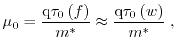 |
(1.128) |
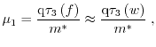 |
(1.129) |
 |
(1.130) |
However, these simple empirical transport models did not deliver satisfactory
results especially in the high field regime. Furthermore, a consistent comparison with
other methods as for instance Monte Carlo simulations
is difficult, because the transport model does
not reproduce the Monte Carlo results in the homogeneous
case [21].
In [112] a transport parameter model based on homogeneous fullband Monte Carlo tables has been
introduced. Here, all higher-order transport parameters
are extracted for different doping concentrations and for different driving
forces. The transport parameters are then considered in the macroscopic
transport models as a function of the average energy. Since all transport
parameters are obtained from Monte Carlo simulations the transport models are free of
fit parameters. Macroscopic models based on Monte Carlo data improves its counterpart models
based on empirical models significantly, both in terms of numerical stability
and in the agreement with Monte Carlo device simulations, as will be demonstrated in
the next chapter.
1.4.4 Monte Carlo Method
The Monte Carlo MC method is a statistical approach to solve
the BTE equation [113,114,115,116,117]. The procedure
does not aim at solving differential equations as described above,
but to observe the trajectories of carriers as they move through a device under
the influence of a driving field and scattering forces [1]. The method is
illustrated in Fig. 1.17. The momentum of a particle is set as an initial condition.
Pseudo-random numbers define the time of free flight of the particles as well as the scattering events.
The simulation converges, when the statistical error of the quantities is under
a certain limit. During convergence transport parameters
like the carrier mobility or higher-order transport parameters can be
extracted.
An advantage of this approach is that all kind of scattering
mechanisms including for instance optical, acoustical phonon scattering
and a general band structure can be modeled very precisely.
Thus, the method is often used as a benchmark for computationally less
expensive transport models. The disadvantage of this statistical approach is that
the error bound of a quantity goes with
 , with
  describing the number of random events. Therefore, with the
increased accuracy of the factor
describing the number of random events. Therefore, with the
increased accuracy of the factor  , the number of scattering events
increases with
, the number of scattering events
increases with
 [118]. The consequence is that the
simulation time increases as well. Therefore, for engineering applications, macroscopic transport models
based on the method of moments, which are computationally much less expensive, are more suitable than the MC technique.
[118]. The consequence is that the
simulation time increases as well. Therefore, for engineering applications, macroscopic transport models
based on the method of moments, which are computationally much less expensive, are more suitable than the MC technique.
Figure 1.17:
Flowchart of a MC Simulation (after [1])
|
|
As displayed in Fig. 1.17, the free flight is an important part
of the MC simulation.
The coordinates of a moving particle in phase space with an applied electric field in
 can be written as
 denotes the conduction band edge, whereas
 is the effective mass
of the electrons and holes, respectively.
The scattering rates
is the effective mass
of the electrons and holes, respectively.
The scattering rates
 of the carriers are indirectly proportional to the duration
of the free flight [22]
of the carriers are indirectly proportional to the duration
of the free flight [22]
The sum includes all scattering mechanisms
 , where the summation of
 denotes
the free flight. The probability of the carrier movement not being affected by the first
collision between
and
denotes
the free flight. The probability of the carrier movement not being affected by the first
collision between
and
 is the scattering rate times the
probability that it survives until the time
[119].
For a random number generator that produces uniformly distributed numbers between
is the scattering rate times the
probability that it survives until the time
[119].
For a random number generator that produces uniformly distributed numbers between
![$ \ensuremath{u}{\;}\in[0,1]$](img428.png) , the collision times can be expressed as [120]
, the collision times can be expressed as [120]
 denotes a constant scattering rate and
 are random
numbers.
Equation (1.134) is a very simple description of the free flight. In
real semiconductor devices the scattering rates are energy dependent. Hence,
equation (1.134) must be rewritten to acknowledge this
fact. This can be done by introducing the so called self-scattering
are random
numbers.
Equation (1.134) is a very simple description of the free flight. In
real semiconductor devices the scattering rates are energy dependent. Hence,
equation (1.134) must be rewritten to acknowledge this
fact. This can be done by introducing the so called self-scattering
 . The
. The
 is
defined as
is
defined as
Note that
is energy dependent. Finally, the total
scattering rate
(
 ) remains
constant, so the simple equation (1.134) can be applied.
It is important that the self-scattering does not influence the trajectories.
Hence, the carriers momentum of a self-scattering event must be unchanged.
Equations (1.131) and (1.132) determine the free flight of the
carriers in an electric field. The Monte Carlo method defines the
correct scattering events as follows:
After the free flight a new scattering event can be obtained in the range
) remains
constant, so the simple equation (1.134) can be applied.
It is important that the self-scattering does not influence the trajectories.
Hence, the carriers momentum of a self-scattering event must be unchanged.
Equations (1.131) and (1.132) determine the free flight of the
carriers in an electric field. The Monte Carlo method defines the
correct scattering events as follows:
After the free flight a new scattering event can be obtained in the range
 |
(1.136) |
 characterizes the total scattering rate
according to equation (1.133) divided by the self-scattering rate before the scattering
event.
characterizes the total scattering rate
according to equation (1.133) divided by the self-scattering rate before the scattering
event.
 is defined via (1.133) divided by
the self-scattering rate, whereas
is a uniform random number between
is defined via (1.133) divided by
the self-scattering rate, whereas
is a uniform random number between
 and
and
 .
The relaxation times can be calculated via Fermi's golden rule [1]
.
The relaxation times can be calculated via Fermi's golden rule [1]
(1.138) is the rate at which carriers with a specific
momentum
 and spin up scatter to any other state. In the sequel,
the scattering at the interface based on (1.137)
and (1.138) will be discussed, which is an important
inversion layer effect.
and spin up scatter to any other state. In the sequel,
the scattering at the interface based on (1.137)
and (1.138) will be discussed, which is an important
inversion layer effect.
As pointed out in [22], the scattering
events calculated with the random procedure explained above are in very good
agreement with the experiment.
The Monte Carlo method allows to evaluate averages of microscopic quantities as defined
in equation (1.69). Assuming an ensemble of
 independent and
identical particles, the estimation of an expected value based on an ensemble
average can be expressed as [112,121]
independent and
identical particles, the estimation of an expected value based on an ensemble
average can be expressed as [112,121]
where
 is the macroscopic quantity and
is the corresponding
microscopic counterpart.
is the macroscopic quantity and
is the corresponding
microscopic counterpart.
 is the statistical weight and
 denotes the
state of the jth carrier. The weight
is defined as
denotes the
state of the jth carrier. The weight
is defined as
 and and  |
(1.140) |
The Monte Carlo simulator used in this work, the so called before-scattering method
is used [122]. Here, the averages are calculated at the end of the
free flight. Hence, equation (1.139) is used right before the next scattering
event.
The relaxation times in a Monte Carlo simulator can be obtained as [123]
 |
(1.141) |
 is the equilibrium energy. Only
depends
on the band structure.
For the energy relaxation times, the equilibrium energy
is defined as [123]
is the equilibrium energy. Only
depends
on the band structure.
For the energy relaxation times, the equilibrium energy
is defined as [123]
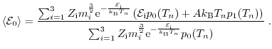 |
(1.142) |
is a dimension factor, whereas
 and
and
 are
polynomials considering the non-parabolicity of the band
structure [123]. The summation index
runs over all valleys in
the material. In the case of silicon the index
is in the range of
to
are
polynomials considering the non-parabolicity of the band
structure [123]. The summation index
runs over all valleys in
the material. In the case of silicon the index
is in the range of
to
 .
In a single valley, the equilibrium energy for three-dimensions can be calculated as
.
In a single valley, the equilibrium energy for three-dimensions can be calculated as
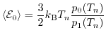 |
(1.143) |
The mobilities for the six moments model can be obtained from the homogeneous macroscopic transport
model as
 is the electric field, the index
denotes the dimension
of the electron gas, and in the numerators of equation (1.144),
there are the odd moments of the BTE as explained in the previous section.
Hence, the mobilities can be calculated as a post-processing step.
is the electric field, the index
denotes the dimension
of the electron gas, and in the numerators of equation (1.144),
there are the odd moments of the BTE as explained in the previous section.
Hence, the mobilities can be calculated as a post-processing step.
1.4.5 Spherical Harmonics Expansion
The Spherical Harmonics Expansion (SHE) procedure is a numerical method for solving
the BTE. It gives approximate deterministic solutions of the
BTE by an expansion of the distribution function
in the
-space
into spherical harmonic functions
 [124]. As will be demonstrated the
SHE procedure reproduces the results obtained from MC quite well with
less computational effort.
[124]. As will be demonstrated the
SHE procedure reproduces the results obtained from MC quite well with
less computational effort.
Spherical harmonic functions are defined
as [125,126]
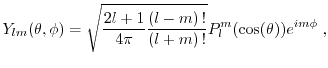 |
(1.145) |
with
 as the associated Legendre polynomial. The indices
 and
are defined in the range
and
are defined in the range
 and
and
 respectively.
Furthermore, the spherical harmonics are orthogonal,
respectively.
Furthermore, the spherical harmonics are orthogonal,
normalized and complex valued [127]. The second term with the primed indices
of (1.146) is the conjugate complex term of
,
whereas
 is defined as
 .
.
For instance the spherical harmonic functions
 ,
,  ,
,  , and
, and
 can be expressed as
is a sphere, while
and
are visualized in Fig. 1.18.
Figure 1.18:
and
in polar coordinates
|
|
Note that for rotational symmetry in the
direction, the
spherical harmonic function is reduced to
the associated Legendre polynomials.
The distribution function can be now expanded as
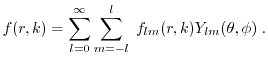 |
(1.148) |
The coefficients
 are given by
The fluxes for a three-dimensional electron gas as defined in (1.83) can be
now expressed as
The next step is to apply the SHE method to the stationary BTE. For the
sake of clarity, the transport direction of the carriers is assumed just
along the
coordinate and a parabolic band structure is taken into
account. Hence, the
expansion (1.149) reduces to
where the angle
 is specified by the direction of the electric
field and the
is specified by the direction of the electric
field and the
 are the Legendre polynomials. Before
substituting the distribution function with spherical harmonics, a variable
transformation from
-space into
-space is performed. The
transformation into the
-space has many advantages, e.g. in equilibrium,
the distribution function is isotropic on equienergy
surfaces [127]. Inserting the expansion (1.151) into
the BTE, one can obtain the BTE expressed by the SHE [128,129]. The first two lowest order expansions can be written as
are the Legendre polynomials. Before
substituting the distribution function with spherical harmonics, a variable
transformation from
-space into
-space is performed. The
transformation into the
-space has many advantages, e.g. in equilibrium,
the distribution function is isotropic on equienergy
surfaces [127]. Inserting the expansion (1.151) into
the BTE, one can obtain the BTE expressed by the SHE [128,129]. The first two lowest order expansions can be written as
 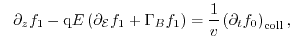 |
(1.152) |
 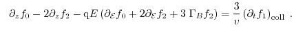 |
(1.153) |
For
 , the result is an exact solution of the
BTE. In Fig. 1.20, a velocity profile of an
structure calculated with a MC simulation and with SHE simulations
taking several Legendre polynomials into account is shown. The result is different
from the MC simulation considering just one Legendre polynomial, whereas
for at least 9 polynomials, both simulations are in good
agreement. Therefore, the SHE simulation is a good benchmark alternative to the Monte Carlo
technique considering enough polynomials.
, the result is an exact solution of the
BTE. In Fig. 1.20, a velocity profile of an
structure calculated with a MC simulation and with SHE simulations
taking several Legendre polynomials into account is shown. The result is different
from the MC simulation considering just one Legendre polynomial, whereas
for at least 9 polynomials, both simulations are in good
agreement. Therefore, the SHE simulation is a good benchmark alternative to the Monte Carlo
technique considering enough polynomials.
The question may arise about the relation of the SHE to macroscopic models as
e.g. the drift-diffusion model. The answer to this question will be discussed
in the following.
Assuming a homogeneous, stationary system with an applied electric field
 , the macroscopic relaxation time approximation on the right hand side of the
BTE, parabolic bands, and the diffusion
approximation [51], the BTE can be written as
, the macroscopic relaxation time approximation on the right hand side of the
BTE, parabolic bands, and the diffusion
approximation [51], the BTE can be written as
To derive an expression for the anti-symmetric part of the distribution
function
, which is the important part for systems within non-equilibrium
conditions, the distribution function
can be split into a symmetric
part
and
. Due to the assumption of the diffusion approximation
which states that the system is not very far away
from equilibrium. The equation (1.154) can now be used to derive an
expression for the anti-symmetric part
[1]
Figure 1.19:
A comparison of the low and high-field mobility as a function
of the doping in the bulk calculated with the SHE method and the
drift-diffusion model. In the SHE simulation, only the first Legendre
polynomial has been taken into account.
|
|
Figure 1.20:
The velocity profile of an
structure calculated with a device MC
simulation and with a SHE simulator taking 1, 5, 9, and 15
Legendre polynomials (LP) into account.
|
|
Inserting equation (1.156) into (1.150) the drift term of the
drift-diffusion model is obtained.
Hence, taking just the first Legendre polynomial of the SHE, in a homogeneous
system within the low-field regime, the results of the SHE are equal to the
results from drift-diffusion simulations.
In Fig. 1.19, the low-field and the high-field mobility calculated
with a SHE simulator and a standard
drift-diffusion model as a function of the doping concentration is shown. In the SHE
simulator, only the
first Legendre polynomial has been taken into account. The results of the two
simulations show a very good agreement in the low-field regime, whereas the
assumptions stated above are not valid anymore for high-fields. The situation changes taking more than one Legendre polynomial into account.
As demonstrated in Fig. 1.20, the SHE method is in very good
agreement with MC simulations when at least
 Legendre
polynomials are considered. Due to the good agreement with MC simulations in short channel
devices and to the shorter simulation time of the SHE method compared
to MC, the SHE method is used as a reference solution for the
derived three-dimensional higher-order macroscopic transport models in the next chapter.
Legendre
polynomials are considered. Due to the good agreement with MC simulations in short channel
devices and to the shorter simulation time of the SHE method compared
to MC, the SHE method is used as a reference solution for the
derived three-dimensional higher-order macroscopic transport models in the next chapter.
Next: 2. The Three-Dimensional Electron
Up: Dissertation Martin-Thomas Vasicek
Previous: List of Figures
M. Vasicek: Advanced Macroscopic Transport Models
![\includegraphics[width=0.5\textwidth]{rot_figures_left/simulation/subband_diff/subb_diff_ana.eps}](img112.png)
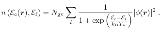
![\includegraphics[width=0.5\textwidth]{rot_figures_left/simulation/transport/vmc2deg/wave_conduction.eps}](img118.png)
![\includegraphics[width=0.5\textwidth]{rot_figures_left/simulation/distribution/distribution.eps}](img129.png)
 and
and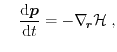
![\includegraphics[width=0.5\textwidth]{figures/svg/trajectories.eps}](img156.png)
![\includegraphics[width=0.5\textwidth]{figures/svg/band_structure_si.eps}](img178.png)
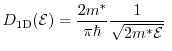 ,
, 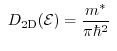 , and
, and 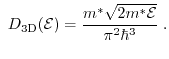
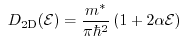 , and
, and 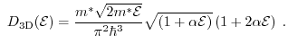
![\includegraphics[width=0.5\textwidth]{rot_figures_left/conferences/sispad2007/pop1_2_color.ps}](img194.png)
![\includegraphics[width=0.5\textwidth]{rot_figures_left/conferences/sispad2007/vel_color.ps}](img195.png)
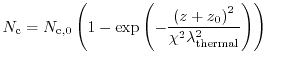 with
with 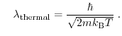
![\includegraphics[width=0.5\textwidth]{rot_figures_left/simulation/quantum_correction/sg_ccn_1.0V/quantum_correction.ps}](img264.png)

 , and
, and 
![\includegraphics[width=0.5\textwidth]{rot_figures_left/simulation/transport/MCdata/Si/kurtosis_nice.eps}](img382.png)
![\includegraphics[width=0.5\textwidth]{rot_figures_left/simulation/transport/nin/closure_M6EEE.eps}](img389.png)
![\includegraphics[width=0.5\textwidth]{rot_figures_left/simulation/transport/MCdata/monju/kur_max.eps}](img390.png)
![\includegraphics[width=0.5\textwidth]{rot_figures_left/simulation/transport/MCdata/monju/distri_TL.eps}](img391.png)
![\includegraphics[width=0.5\textwidth]{rot_figures_left/simulation/transport/closure_2D/2D_closure.eps}](img392.png)
![\includegraphics[width=0.5\textwidth]{rot_figures_left/simulation/transport/nonparafac_color.eps}](img397.png)
 ,
,  , and
, and 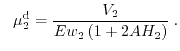
 ,
,  ,
,  , and
, and 
![\includegraphics[width=0.5\textwidth]{rot_figures_left/simulation/SHE-DD/mobility.eps}](img495.png)
![\includegraphics[width=0.5\textwidth]{rot_figures_left/simulation/transport/nin/velocity_all.eps}](img496.png)
![\includegraphics[width=14.5cm]{figures/svg/transport_models.eps}](img75.png)
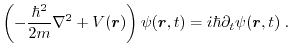
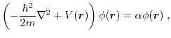
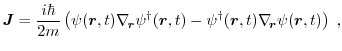
![\includegraphics[width=11.5cm]{figures/svg/quantum_confinement.eps}](img106.png)
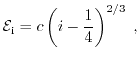
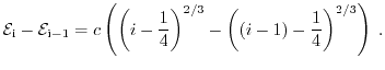
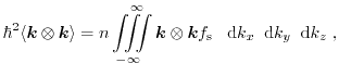
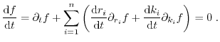
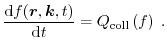
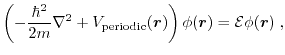
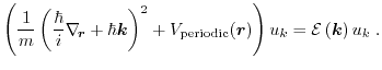
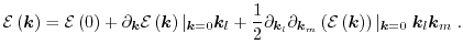
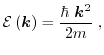
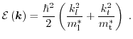
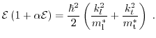
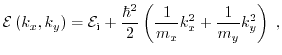
![\includegraphics[width=0.5\textwidth]{figures/svg/subband_ladder.eps}](img193.png)
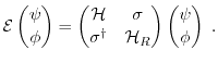
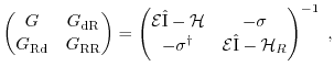
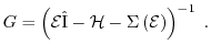
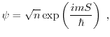

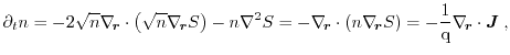
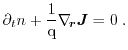
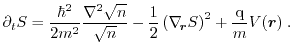
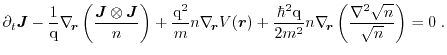
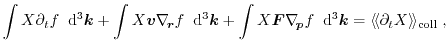
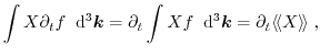
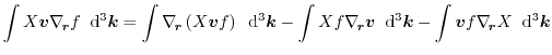

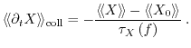
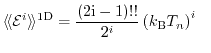 ,
,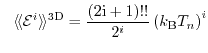
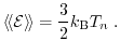
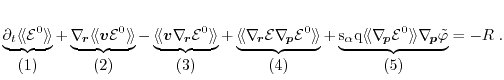
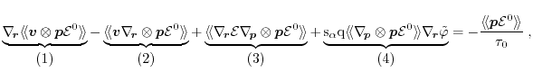

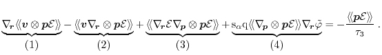
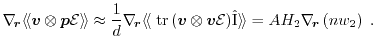

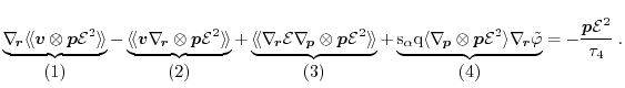
![\includegraphics[width=0.5\textwidth]{figures/svg/MonteCarlo.eps}](img413.png)
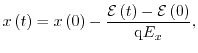
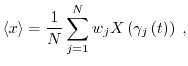
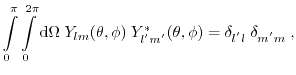
![\includegraphics[width=0.5\textwidth]{figures/simulation/SHE-DD/Y-1-0-spheric.eps}](img477.png)
![\includegraphics[width=0.5\textwidth]{figures/simulation/SHE-DD/Y-2-0-spheric.eps}](img478.png)