Subsections

• 2.5.1 Boundary Conditions and the Complete System
• 2.5.2 Extension for Higher-Order Transport Models

2.5 Derivation of the Complex-Valued Small-Signal System

In order to derive the complex-valued small-signal system based on the ${\textrm{S}^3\textrm{A}}$ approach, the equations (2.21), (2.22), and (2.23) can be symbolically written as [90]:

$${ F_{\psi}(\psi, n, p) = 0\ ,$$ (2.117)

$$F_{n}(\psi, n, p) = \displaystyle \frac{\displaystyle \partial G_{n}(n(t))}{\displaystyle \partial t}\ ,$$ (2.118)

$$F_{p}(\psi, n, p) = \displaystyle \frac{\displaystyle \partial G_{p}(p(t))}{\displaystyle \partial t}\ . {$$ (2.119)

For the derivation of the linear small-signal system, the following time-dependent functions

$${ \psi(t) = \psi_0 + \ensuremath{\underline{\psi}} \displaystyle \displaystyle e^{\ensuremath{\mathrm{j}}\omega t}\ ,$$ (2.120)

$$n(t) = n_0 + \ensuremath{\underline{n}} \displaystyle \displaystyle e^{\ensuremath{\mathrm{j}}\omega t}\ ,$$ (2.121)

$$p(t) = p_0 + \ensuremath{\underline{p}} \displaystyle \displaystyle e^{\ensuremath{\mathrm{j}}\omega t}\ , {$$ (2.122)

are substituted into the equations (2.117), (2.118), and (2.119) to obtain

$${ F_{\psi}(\psi_0 + \ensuremath{\underline{\psi}} \displaystyle \... ...ne{p}} \displaystyle \displaystyle e^{\ensuremath{\mathrm{j}}\omega t}) = 0 \ ,$$ (2.123)

$$F_{n}(\psi_0 + \ensuremath{\underline{\psi}} \displaystyle \displ... ...laystyle e^{\ensuremath{\mathrm{j}}\omega t})}{\displaystyle \partial t} = 0\ ,$$ (2.124)

$$F_{p}(\psi_0 + \ensuremath{\underline{\psi}} \displaystyle \displ... ...aystyle e^{\ensuremath{\mathrm{j}}\omega t})}{\displaystyle \partial t} = 0\ .{$$ (2.125)

The zero subscript stands for the steady-state operating point of the device. The time derivatives of the $G$ functions in (2.118) and (2.119) are calculated using the chain rule as follows:

$${ \displaystyle \frac{\displaystyle \partial G_{n}(n(t))}{\displa... ...suremath{\mathrm{j}}\omega \displaystyle e^{\ensuremath{\mathrm{j}}\omega t}\ ,$$ (2.126)

$$\displaystyle \frac{\displaystyle \partial G_{p}(p(t))}{\displays... ...uremath{\mathrm{j}}\omega \displaystyle e^{\ensuremath{\mathrm{j}}\omega t}\ .{$$ (2.127)

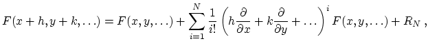
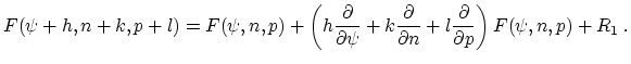
To obtain the linearized version of (2.117), (2.118), and (2.119), a Taylor series expansion is performed, which is generally defined for a function with several unknowns as follows [29]:

$${ F(x + h, y + k, \ldots) = F(x, y, \ldots) + \sum_{i=1}^{N} \fra... ...rtial }{\displaystyle \partial y} + \ldots \right)^i F(x, y, \ldots) + R_N\ , }$$ (2.128)

where $R_N$ is the remainder term of the approximation. This formula can be specialized for the three unknowns $\psi$, $n$, and $p$, and termination after the linear part ($i=1$) resulting in the small-signal approximation:

$${ F(\psi + h, n + k, p + l) = F(\psi, n, p) + \left(h \displaysty... ...splaystyle \partial }{\displaystyle \partial p} \right) F(\psi, n, p) + R_1\ .}$$ (2.129)

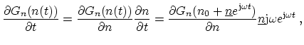
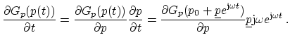
By applying (2.129) for the functions $F$ of equations (2.123), (2.124), and (2.125) with the functions (2.120), (2.121), and (2.122), the following approximation is derived:

$$F_{}(\psi_0 + \ensuremath{\underline{\psi}} \displaystyle \displa... ...nderline{p}} \displaystyle \displaystyle e^{\ensuremath{\mathrm{j}}\omega t}) =$$ (2.130)

$$= \underbrace{F_{}(\psi_0,n_0,p_0)}_{\text{dc solution}} + \displ... ...le e^{\ensuremath{\mathrm{j}}\omega t}F_{}\right]}{\displaystyle \partial p}\ .$$ (2.131)

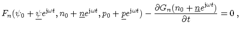
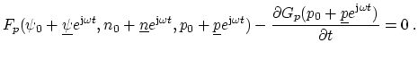
If this approximation is substituted into equations (2.123), (2.124), and (2.125), the resulting equation system reads

$$0 = \underbrace{F_{\psi}(\psi_0,n_0,p_0)}_{\text{dc solution}} +\... ...isplaystyle \partial F_{\psi}}{\displaystyle \partial p} \end{array} \right]\ ,$$ (2.132)

$$0 = \underbrace{F_{n}(\psi_0,n_0,p_0)}_{\text{dc solution}} +\dis... ...{\displaystyle \partial F_{n}}{\displaystyle \partial p} \end{array} \right]\ ,$$ (2.133)

$$0 = \underbrace{F_{p}(\psi_0,n_0,p_0)}_{\text{dc solution}} +\dis... ...ystyle \partial G_{p}}{\displaystyle \partial p} \right) \end{array} \right]\ .$$ (2.134)

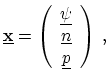
According to equations (2.99), (2.100), and (2.101), the steady-state solutions are equal to zero. This linear equation system can be written in the following matrix notation [127], where the subscript $\mathrm{dc}$ emphasizes that all derivatives are evaluated at the steady-state operating point:

$$\left[ \begin{array}{lll} \displaystyle \frac{\displaystyle \part... ...h{\underline{n}} \\ [2mm] \ensuremath{\underline{p}} \end{array} \right] = 0\ .$$ (2.135)

The real-valued part of the system matrix equals the Jacobian matrix as shown in (2.108). For that reason, the assembly of this part of the matrix can be performed in exactly the same way as for steady-state analysis. The complex-valued contributions are then added by the transient models. As a consequence, the real-valued part can be stored during a frequency stepping since only the complex-valued part is modified.

As already discussed in Section 2.3.1, the exact Jacobian matrix can be replaced by a simpler matrix. Since the solution of the ${\textrm{S}^3\textrm{A}}$ small-signal system does not involve an iterative process but is based on the linearization of the device, it is absolutely necessary to take all derivatives into account. If the simulator offers the possibility to skip several entries (for example iteration schemes, see Section 3.6.4), it has to be ensured that the complex-valued system matrices contain all necessary entries. The same problem occurs while iteratively solving the complex-valued equation system. The preconditioner has to be configured in such a way that no entries are removed (see Section 5.2.5).

2.5.1 Boundary Conditions and the Complete System

In contrast to the Newton procedure, the right-hand-side vector is mostly zero. The small-signal Neumann boundary conditions are the same as during steady-state analysis. The frequency-independent boundary conditions for $n$ and $p$ are zero, because the derivatives vanish in the Taylor series expansion of the contact control function. Real- or complex-valued Dirichlet boundary conditions for $\psi$ can be used to excite the system.

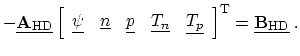
After the complete complex-valued linear system for a small-signal analysis is assembled, the following parts can be identified:

$$- \left[ \ensuremath{\mathbf{J}} + \ensuremath{\mathrm{j}}\omega ... ...\ensuremath{\mathbf{x}}}} = \ensuremath{\underline{\ensuremath{\mathbf{b}}}}\ ,$$ (2.136)

where $\mathbf{J}$ is the real-valued Jacobian as shown in (2.108) and (2.135), $\mathbf{C}$ contains the contributions of the time-dependent nonlinear $G$ functions, $\underline{\ensuremath{\mathbf{x}}}$ is the complex-valued solution vector

$$\ensuremath{\underline{\ensuremath{\mathbf{x}}}} = \left( \begin{... ... \ensuremath{\underline{n}} \\ \ensuremath{\underline{p}} \end{array}\right)\ ,$$ (2.137)

and $\underline{\ensuremath{\mathbf{b}}}$ the complex-valued right-hand-side vector.

2.5.2 Extension for Higher-Order Transport Models

The small-signal system for the energy-transport transport model reads as follows:

$$- \ensuremath{\ensuremath{\underline{\ensuremath{\mathbf{A_\mathr... ... = \ensuremath{\ensuremath{\underline{\ensuremath{\mathbf{B_\mathrm{HD}}}}}}\ .$$ (2.138)

with

$$\ensuremath{\ensuremath{\underline{\ensuremath{\mathbf{A_\mathrm{... ...tyle \partial G_{n}}{\displaystyle \partial n} \\ [4mm] \end{array} \right] \ .$$ (2.139)

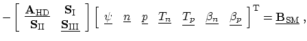
With matrix $\ensuremath{\underline{\ensuremath{\mathbf{A_\mathrm{HD}}}}}$ from (2.139), the small-signal system for the six moments transport models is eventually given by

$$- \left[ \begin{array}{cc} \ensuremath{\ensuremath{\underline{\en... ...= \ensuremath{\ensuremath{\underline{\ensuremath{\mathbf{B_\mathrm{SM}}}}}} \ ,$$ (2.140)

with

$$\ensuremath{\mathbf{S}}_\mathrm{I}^\mathrm{T} = \left[ \begin{arr... ...math{T_p}}}{\displaystyle \partial \ensuremath{\beta_p}} \end{array} \right]\ ,$$ (2.141)

$$\ensuremath{\mathbf{S}}_\mathrm{II} = \left[ \begin{array}{lllll}... ...math{\beta_p}}}{\displaystyle \partial \ensuremath{T_p}} \end{array} \right]\ ,$$ (2.142)

$$\ensuremath{\underline{\ensuremath{\mathbf{S}}_\mathrm{III}}} = \... ...{\beta_p}}}{\displaystyle \partial \ensuremath{\beta_p}} \end{array} \right]\ .$$ (2.143)