It is well-known that adaptive finite element methods based on an a
posteriori error estimator have become very important in scientific and
engineering computing. The numerical procedures for practical problems in
physics or engineering, such as semiconductor processing and device simulation,
often encounter the difficulty that the overall accuracy of the numerical
approximation is deteriorated by local singularities. An obvious remedy is to
refine the discretization near critical regions. The question is how to
identify those regions and how to obtain a good balance between refined and
non-refined regions, such that the local accuracy guarantees an desired
overall accuracy [73].
A lot of theoretical work with different mathematical and engineering aims has
been carried out over the last two decades, see, for
example [74,75,76,77,78,79] and references
cited therein. One class of a posteriori error estimators is the gradient recovery
type, see e.g. [80,81]. Although its mathematical analysis is
still incomplete, the gradient recovery error estimator has been widely used
in adaptive finite element calculation and software engineering. In the
following an error estimator is presented which follows the spirit of gradient
recovery estimators. The basic idea is to find an estimator that considers the
change of the calculated gradient from one element to a neighboring one.
For the following a linear basis function approach as described in
Section 3.1.3 for the interpolation over a ![]() -simplex of scalar data
in a 0
-face relation, cf. Figure 3.1(a) is assumed. The gradient
field can than be calculated as described in Section 3.3.1,
Equation (3.16). Since the vector field (3.16) is
piecewise constant, it is obvious that strong variations of the gradient from
one element to an adjacent one yield an approximation error compared to the
proper continuous gradient field.
-simplex of scalar data
in a 0
-face relation, cf. Figure 3.1(a) is assumed. The gradient
field can than be calculated as described in Section 3.3.1,
Equation (3.16). Since the vector field (3.16) is
piecewise constant, it is obvious that strong variations of the gradient from
one element to an adjacent one yield an approximation error compared to the
proper continuous gradient field.
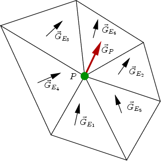
In order to rate the gradient discretization error a
posteriori, linear basis functions, see Equation (3.6) are used,
to construct a piecewise linear gradient field. To accomplish this idea it
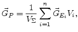
is required to assign an estimated gradient vector - vertex gradient
vector -
![]() to each vertex of the mesh. The vertex gradient vector
is an arithmetic, volume weighted, average vector of all element gradient
vectors
to each vertex of the mesh. The vertex gradient vector
is an arithmetic, volume weighted, average vector of all element gradient
vectors
![]() attached to the vertex, yielding
attached to the vertex, yielding
 |
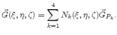
The piecewise linear gradient field can be constructed from (4.2) and (3.6) as
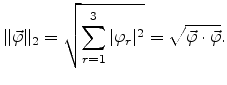
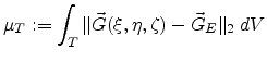
To calculate the error ![]() related to an element
related to an element ![]() , we accumulate
Equation (4.4) applied to the difference between the vector
fields (3.16) and (4.3)
over the element, i.e.,
, we accumulate
Equation (4.4) applied to the difference between the vector
fields (3.16) and (4.3)
over the element, i.e.,
The error estimation given by (4.5) assigns each discretization
element of the domain an error value. The smaller the error value, the
better the piecewise constant vector field fits the piecewise linear one. It is
obvious that a strong variation of the gradient from one element to an adjacent
one adds to an approximation error. So it is in the nature of this error
estimator to detect those regions with higher variation of the gradient.