Subsections

• 3.3.1 Gradient Field
• 3.3.2 Propaedeutic Example

3.3 Gradient Refinement Method

In Section 3.2 the so-called layer refinement method was presented. For this method the solution of the Laplace equation was used as approximation of the surface distance field and an element grading example was shown, where mesh elements are mostly isotropic. Now the layer refinement method is extended by introducing a primary stretching direction. This direction is aligned to the direction of the gradient field of the initial scalar data field stored on the mesh. This yields the name gradient refinement method.

3.3.1 Gradient Field

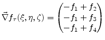
With the help of linear weighting functions, it is possible to calculate the gradient of a given scalar data field on a tetrahedral mesh element. It is in the nature of this approach, that the gradient is constant over the element (vector data $3$ -face relation, cf. Figure 3.1(b) and Figure 3.2(d)) and varies from element to element, so the gradient field is piecewise constant.

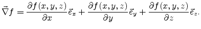
The gradient $\vec{\nabla} f =$   grad$f$ of a scalar field $f=f(x,y,z)$ in Cartesian coordinates is given by

$$\vec{\nabla} f = \frac{\partial f(x,y,z)}{\partial x}\vec{e}_x+ \... ... f(x,y,z)}{\partial y}\vec{e}_y+ \frac{\partial f(x,y,z)}{\partial z}\vec{e}_z.$$ (3.13)

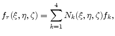
Using linear weighting functions on the three-dimensional unit simplex, which are given by Equation (3.6), discussed in Section 3.1.3, allow a linear approximation of the scalar field over the element in the form

$$f_{\tau}(\xi,\eta,\zeta) = \sum_{k=1}^{4} N_{k}(\xi,\eta,\zeta)f_{k},$$ (3.14)

where $f_{k}$ denotes the scalar value on the $k^{th}$ 0 -face of the standard $3$ -simplex $\tau$ . Applying (3.13) to the linear approximation $f_{\tau}$ , given by (3.14), the gradient expressed in local coordinates, using linear weighting functions (3.6), results to

$$\vec{\nabla} f_{\tau}(\xi,\eta,\zeta) = \begin{pmatrix}-f_{1}+f_{2} \ -f_{1}+f_{3} \ -f_{1}+f_{4} \end{pmatrix}$$ (3.15)

for the gradient of the spatial discretization element. Using the inverse of the transposed Jacobian matrix the gradient can be transformed to global coordinates by

$$\vec{\nabla} f_{\tau}(x,y,z)= (\mathbf{J}^{T})^{-1}\cdot \vec{\nabla} f_{\tau}(\xi,\eta,\zeta).$$ (3.16)

The gradient expressed through Equation (3.16) is constant over an element $\tau$ and forms a piecewise constant gradient field which gives a granular approximation of the proper gradient field given by Equation (3.13).

However, for the gradient refinement method the basic idea is to use the gradient of a given scalar data field stored on the initial mesh to define an anisotropic refinement metric. This metric is used for an anisotropic tetrahedral bisection process as described in Section 2.3.1 and Section 2.3.2. If the gradient given by Equation (3.15) vanishes completely, the gradient is set to $\vec{\nabla}f_{\tau}(\xi,\eta,\zeta) = {3}^{-1/2}(1,1,1)^T$ .

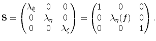
As seen in Section 2.3.1, a three-dimensional tensor-based metric function $\mathbf{M}$ can be defined as a combination of rotation matrix $\mathbf{R}$ and dilation matrix $\mathbf{S}$ . The idea is to use the direction of the gradient field as the primary stretching direction. The dilation factor itself is dependent on the initial scalar data field, stored on the mesh. For this refinement method the dilation function is defined slightly differently compared to the layer refinement method, described in the previous section (cf. Equation (3.11)):

$$\mathbf{S} =\begin{pmatrix}\lambda_{\xi} & 0 & 0 \ 0 & \lambda_{... ...egin{pmatrix}1 & 0 & 0 \ 0 & \lambda_{\eta}(f) & 0 \ 0 & 0 & 1 \end{pmatrix}.$$ (3.17)

One can see that now only $\lambda_{\eta}$ depends on the scalar data field $f(x,y,z)$ stored on the initial mesh. $\lambda_{\xi}$ and $\lambda_{\zeta}$ are set to unity and there is no dilation with respect to the $\xi$ - and $\zeta$ -direction.

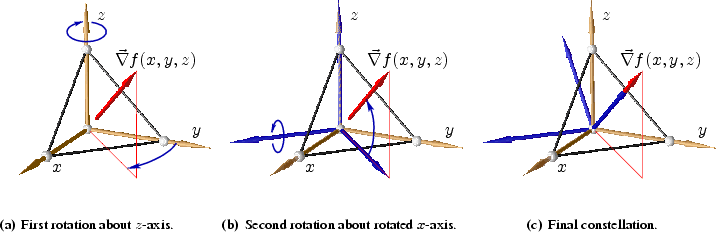
As second step, a directional dependence is introduced by rotating the dilation function so that the $\eta$ -direction is parallel to the direction of the gradient field of $f(x,y,z)$ . To accomplish this task one first has to rotate the three axes of the Cartesian coordinate system $\{\vec{x},\vec{y},\vec{z}\}$ in the way that the new $y$ -axis is parallel to the gradient vector. The evolution of this rotation is illustrated in Figure 3.9, where the gradient vector $\vec{\nabla}f = \operatorname{grad} f$ was calculated on a standard $3$ -simplex. The rotation matrix $\mathbf{R}$ can be easily calculated with Euler rotation angles, see Appendix B.1 for a detailed description.

Figure 3.9: Rotation evolution for the transformation of the dilation function matrix $\mathbf{S}$ demonstrated on the standard $3$ -simplex. The first rotation is around the $z$ -axis and the second is about the rotated $x$ -axis so that the former $y$ -axis is parallel to the direction of the gradient $\vec{\nabla}f$ of the scalar data function $f(x,y,z)$ .

For the dilation function $\lambda_{\eta}$ different features are cogitable. One method is to use the same functional dependence as described in Section 3.2, where the dilation is scalar data dependent, i.e. $\lambda_{\eta} = \lambda(f(x,y,z))$ . But one has to keep in mind that the main difference here is the introduction of a primary stretching direction, i.e. that only the $y$ -axis, which is after the rotation parallel to the direction of the gradient field, related dilation factor $\lambda_\eta$ is functional dependent. All other dilation factors $\lambda_\xi$ and $\lambda_\zeta$ are set to unity as depicted in Equation (3.17).

In the following an example is given where for the dilation function a dependence of an initial scalar data distribution $f(x,y,z)$ is introduced. Here again the data function $f$ is normalized to unity and the same function as depicted in Figure 3.6 can be used for $\lambda_\eta$ .

3.3.2 Propaedeutic Example

In this example a combination between the layer refinement method described in Section 3.2 and the gradient refinement method is chosen. The refinement itself is based on the anisotropic tetrahedral bisection algorithm presented in Section 2.3.2, Table 2.2.

The idea of this example is to produce a fine anisotropic mesh near a particular surface of the mesh domain. The finer region should be limited to a layer with a particular thickness. Isotropic elements should be oriented so that a high mesh density, i.e. edges of short Euclidian length, arises perpendicular to the surface, other directions should be mostly untouched. Figure 3.10(a) show the initial structure where a cubic body (colored green) is covered with an L-shaped mask (colored blue).

Figure 3.10: Example structure of the gradient refinement method, where a cubic body is covered by an L-shaped mask. For the approximation of the surface distance field the solution of the Laplace equation is chosen with Dirichlet boundary conditions. On all other surfaces Neumann boundary conditions are applied. Figure 3.10(c) shows the iso-levels of the Laplace equation solution and Figure 3.10(d) the corresponding gradient field.

For the construction of the dilation function $\lambda_\eta$ , we first solve the Laplace equation, on the initial coarse mesh domain, considering the given appropriate boundary conditions as depicted in Figure 3.10(b). Only the upper part of the cubic body, not covered by the mask, and the opposite boundary hold Dirichlet boundary conditions. The Dirichlet conditions are set as follows: the not covered upper part is set to unity and the opposite plane is set to zero. All other boundaries hold Neumann boundary conditions. The solution of the Laplace equation is the scalar field $f(x,y,z)$ , iso-levels of $f$ , and the corresponding gradient field $\vec{\nabla}f(x,y,z)$ are shown in Figure 3.10(c) and Figure 3.10(d), respectively. Note that the gradient field is orthogonal to the iso-levels.

The next step is to define the dilation function $\lambda_\eta$ in dependence to the solution of the Laplace equation $f(x,y,z)$ in the form $\lambda_\eta = \lambda_\eta(f(x,y,z))$ . As noticed in the preamble of this section, the refinement should cover only a small surface layer with a well defined thickness. This task was already matter of the layer refinement method, described in Section 3.2. The same function as depicted in Figure 3.6 for the dilation function $\lambda_\eta$ is used. Now the dilation function matrix which is given by Equation 3.17 is completely specified.

For the three-dimensional anisotropic tetrahedral bisection algorithm, described in Section 2.3.2, a metric function $\mathbf{M}$ must be specified which is given by a dilation function matrix $\mathbf{S}$ and an additional rotation matrix $\mathbf{R}$ since $\mathbf{M}=\mathbf{R}\mathbf{S}\mathbf{R}^T$ . The rotation matrix can be easily constructed by the rotation evolution depicted in Figure 3.9, so that the new $y$ -axis is parallel to the gradient vector, which is the sine qua non of the gradient refinement method.

Finally, for the anisotropic tetrahedral bisection algorithm an edge refinement criterion, as shown in Table 2.2 and Table 2.3, respectively, has to be specified . Here again (cf. Section 3.2) we use simply an upper limit for the anisotropic length of all mesh edges, so that all edges are refined which overshoot this maximum.

Figure 3.11: The gradient refinement method was chosen to obtain an anisotropic refinement in regions of scalar data values above $70 \%$ of the maximum. For the anisotropic primary stretching direction the gradient field of the Laplace equation solution $f(x,y,z)$ was used. The refinement is limited to the cubic body, the L-shaped mask on top is influenced by mesh conformity reasons only.

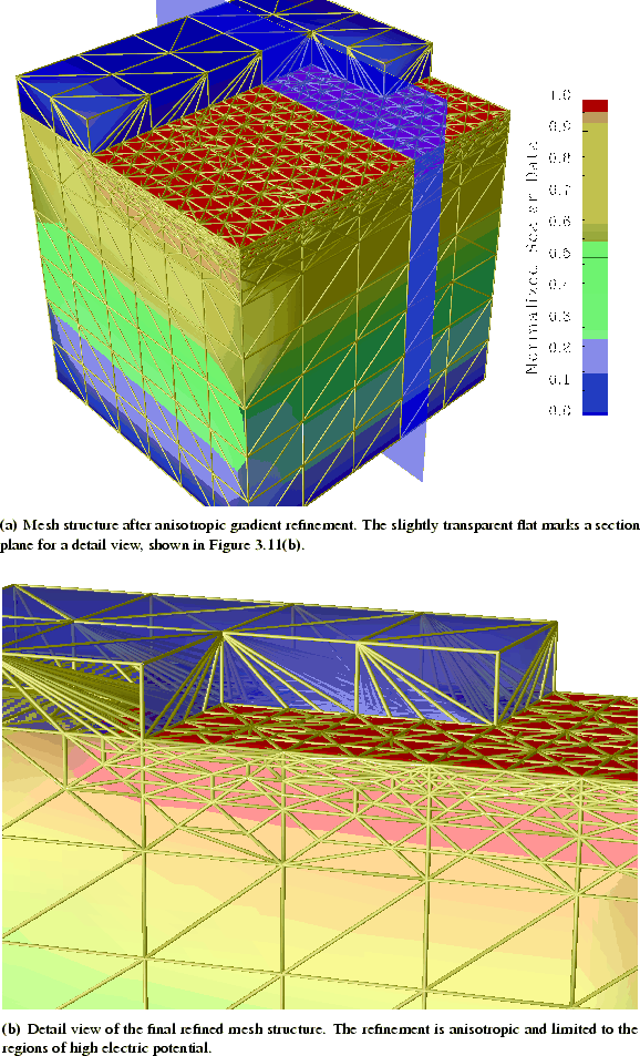Figure 3.11 shows the resulting refined structure. The refinement exhibits an excellent local behavior and covers the whole region where the solution of the Laplace equation $f(x,y,z)$ shows values above $70 \%$ of the maximum. The anisotropy is produced according to the orientation of the gradient field, i.e., along the gradient direction a much higher mesh density appears, all other directions are influenced only slightly. Other regions of the structure are kept totally untouched. Only the mask on top is influenced by the refinement, which is clear since the mesh conformity has to be guaranteed over the whole simulation domain and must not be violated by the refinement procedure.

This example closes the section about the gradient refinement method. Topic of the next section is the so-called Hessian refinement method which can be used to produce anisotropic meshes governed by the second derivatives of an initial scalar data field stored on the mesh.