The idea behind this example is to test the heuristic error estimator described
in Section 4.1 on a bottom-of-the-line case. The chosen diffusion
problem is one-dimensional in its nature but calculated on a three-dimensional
test structure, and with proper chosen boundary conditions, an
analytical solution can be given. This helps to modify the error estimator and
calculate the distance between the piecewise calculated gradient field and the
analytical one, as part of the error estimation. Afterwards an anisotropic
Hessian refinement is applied to see, if a finer mesh really reduces the
estimated error. Finally, the modified error estimator is compared to the
original one given in Section 4.1.
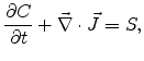
The balance of quantity ![]() in a bounded domain
in a bounded domain ![]() in general form
is given by
in general form
is given by
where ![]() gives the flux,
gives the flux,
![]() is called production rate within
is called production rate within ![]() , and
, and
![]() gives the increase per time of
gives the increase per time of ![]() within
within
![]() . If
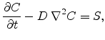
. If ![]() is given by Equation (4.1), then
Equation (4.6) forms a parabolic partial differential equation,
is given by Equation (4.1), then
Equation (4.6) forms a parabolic partial differential equation,
where ![]() denotes the diffusion coefficient. In a first approximation the
diffusion coefficient
denotes the diffusion coefficient. In a first approximation the
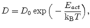
diffusion coefficient ![]() is given by the so-called Arrhenius law,
is given by the so-called Arrhenius law,
where the pre-exponential factor ![]() is a material dependent parameter,
is a material dependent parameter,
![]() is Boltzmann's constant,
is Boltzmann's constant, ![]() the temperature, and
the temperature, and ![]() the activation energy.
the activation energy.
For the
manufacturing cycle of semiconductor devices two conditions of the
source term free Equation (4.7) with ![]() , are important:
, are important:
 .
.
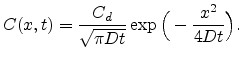
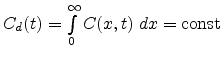
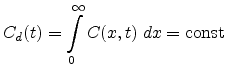
The following deals with the case of ``constant dose'', which is also referred
as so-called drive in diffusion.
For a one-dimensional case under consideration of the following conditions:
The numerical representation of time continuous problems based on FE methods
yields also a discretization in time. Therefore the ``continuous time'' is split
into small slices, named time steps.
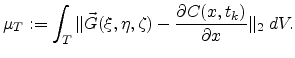
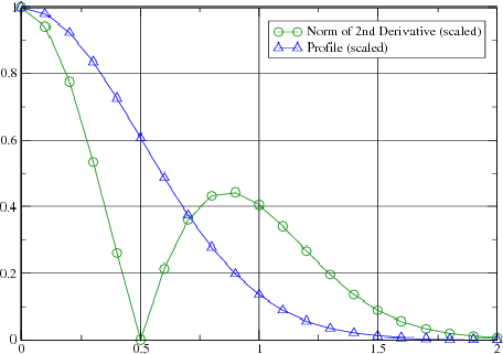
In the following a to unity scaled quantity as temporary result of a drive in
diffusion simulation at the time step ![]() is under examination regarding the
error estimator discussed in Section 4.1. Figure 4.2 shows
the corresponding graph and the scaled norm of the second derivative of the
one-dimensional test case which was applied to a three-dimensional test
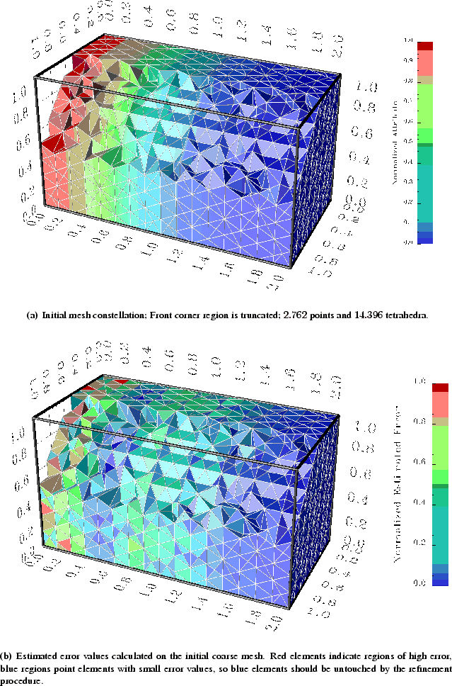
structure depicted in Figure 4.3(a).
is under examination regarding the
error estimator discussed in Section 4.1. Figure 4.2 shows
the corresponding graph and the scaled norm of the second derivative of the
one-dimensional test case which was applied to a three-dimensional test
structure depicted in Figure 4.3(a).
 |
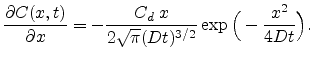
Due to the fact, that an analytical solution of the parabolic partial differential equation is available, the error estimator can be modified in such a way, that the element gradient can directly be compared with the gradient of the analytical solution, which is given by:
The coloration of Figure 4.3(b) gives the normalized estimated error
according to the error estimator presented in Section 4.1 with the
modification expressed through Equation (4.12). Regions
with red colored tetrahedrons indicate that a high error value was
calculated. One can clearly observe that in regions with high curvature,
i.e. with high second derivatives which can be seen as measure for the
curvature of the initial profile (cf. Figure 4.2), a higher error
is located. This note gives rise to the idea that the Hessian refinement method described in
Section 3.4 can produce a finer anisotropic mesh
in the region of higher estimated error. The difference now is that only
those tetrahedra with an error higher than ![]() of the maximum error
are used for refinement and others are untouched. This means that not the whole
structure is involved in the refinement process and the refinement is kept
local.
of the maximum error
are used for refinement and others are untouched. This means that not the whole
structure is involved in the refinement process and the refinement is kept
local.
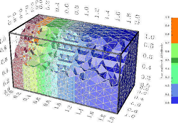
The anisotropic refinement based on the Hessian matrix of the profile takes
place only in regions of high curvature as shown in
Figure 4.4. The anisotropy is mostly restricted to the
![]() -direction of the test structure while other directions are not influenced.
One can clearly observe that the refinement at
-direction of the test structure while other directions are not influenced.
One can clearly observe that the refinement at ![]() is almost zero, which is
forced through the second derivative of the profile which is exactly zero at
is almost zero, which is
forced through the second derivative of the profile which is exactly zero at
![]() . On the left upper end of the structure the mesh granularity in
. On the left upper end of the structure the mesh granularity in
![]() -direction shows the most dense mesh, because of a high curvature of the
profile and, therefore, a high second derivative which yields to a strong
dilation of the anisotropic metric. The region between
-direction shows the most dense mesh, because of a high curvature of the
profile and, therefore, a high second derivative which yields to a strong
dilation of the anisotropic metric. The region between ![]() and
and ![]() shows a high curvature too.
According to the norm of the second derivative, this forming is not as
strong as in the region around
shows a high curvature too.
According to the norm of the second derivative, this forming is not as
strong as in the region around ![]() and, therefore, has less influence on the
refinement procedure.
and, therefore, has less influence on the
refinement procedure.
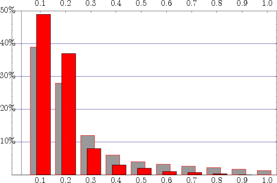
The error estimator was also applied to the refined structure given in
Figure 4.4 and compared to the previous results calculated on
the mostly regular, coarse mesh. The results are shown in Figure 4.5
where the gray-scaled bars reflect the coarse structure, whereas the refined one is
given in red. The error was normalized to the maximum error of the coarse
structure (see Figure 4.3(b)) and divided into ten error classes from
![]() (low error) to
(low error) to ![]() (high error), respectively. Since the number
of tetrahedrons changed after the refinement, the amount regarding the error
class is given in
(high error), respectively. Since the number
of tetrahedrons changed after the refinement, the amount regarding the error
class is given in ![]() . The error estimation is performed with
Equation (4.12) for each element of the domain.
A clear shift towards lower error classes can be observed for the refined
structure. Within the two lowest classes an increase of elements of
approximately
. The error estimation is performed with
Equation (4.12) for each element of the domain.
A clear shift towards lower error classes can be observed for the refined
structure. Within the two lowest classes an increase of elements of
approximately ![]() was reached. All other classes are lowered and the maximum
error class, carrying the highest error of the coarse structure, vanished
completely.
was reached. All other classes are lowered and the maximum
error class, carrying the highest error of the coarse structure, vanished
completely.
The modified error estimator given by Equation (4.12) was also
compared to the original one discussed in Section 4.1 where a
piecewise linear gradient field was constructed of a piecewise constant gradient
field, see Equation (4.5). The difference between those two
estimators is smaller than ![]() of the maximum error value. It
was also observed that for regions of ``smooth'' gradient fields the difference
falls beyond
of the maximum error value. It
was also observed that for regions of ``smooth'' gradient fields the difference
falls beyond ![]() . This observation gives rise to the assumption that the heuristic
error estimator described in Section 4.1 detects excellently regions
of high gradient variations.
. This observation gives rise to the assumption that the heuristic
error estimator described in Section 4.1 detects excellently regions
of high gradient variations.
 |
 |
 |
 and
and