In the following I want to show how the afore said works in detail applied to a tetrahedron.
Figure A.1 shows an arbitrary constellation of four points
![]() which form a tetrahedron. In the following a step by step
recipe is given for applying PCA to this constellation.
which form a tetrahedron. In the following a step by step
recipe is given for applying PCA to this constellation.
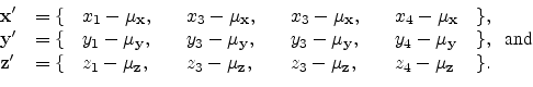
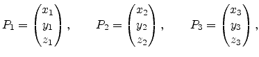
First three sets are formed, namely
![]() ,
,
![]() , and
, and
![]() , by collecting the coordinates of the four tetrahedron
points
, by collecting the coordinates of the four tetrahedron
points
![]() :
:
 and and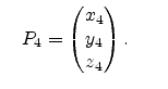 |
(A.12) |
| (A.13) |
For PCA the next step is to subtract the mean from each data set, so three new sets are defined:
Note that the mean value of the three data sets
![]() ,
,
![]() , and
, and
![]() presented in
Equation (A.14) is equal to zero, i.e.
presented in
Equation (A.14) is equal to zero, i.e.
![]() .
.
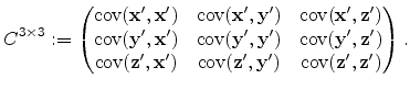
With respect to Equation (A.8) a
![]() covariance matrix is
formed from the three mean adjusted data sets
covariance matrix is
formed from the three mean adjusted data sets
![]() ,
,
![]() , and
, and
![]() , see Equation (A.14).
, see Equation (A.14).
Under the assumption that Equation (A.11) holds, there exist
exact three real eigenvalues ![]() ,
, ![]() , and
, and ![]() (since
the covariance matrix is symmetric) and three corresponding orthogonal
eigenvectors
(since
the covariance matrix is symmetric) and three corresponding orthogonal
eigenvectors ![]() ,
, ![]() , and
, and ![]() . If the three
eigenvalues are not different, the corresponding eigenvectors cannot be
determined uniquely. In this case an arbitrary system of three orthogonal vectors
is used for a so-called ellipsoidal glyph visualization.
. If the three
eigenvalues are not different, the corresponding eigenvectors cannot be
determined uniquely. In this case an arbitrary system of three orthogonal vectors
is used for a so-called ellipsoidal glyph visualization.
![\includegraphics[width=0.23\textwidth]{pics/one-tet.eps}](img573.png)