The most simple way to describe the vertical profile of the dopant
concentration  qualitatively is to utilize a Gaussian distribution
function (2.2-1).
qualitatively is to utilize a Gaussian distribution
function (2.2-1).
The three parameters  ,
,  and
and  are determined by the projected range
 , the standard deviation
  , and the normalization condition
(2.2-2). Using the total implanted dose per unit area
, and the normalization condition
(2.2-2). Using the total implanted dose per unit area  the
concentration is given by (2.2-3).
the
concentration is given by (2.2-3).
We frequently characterize an arbitrary distribution function in
terms of its moments. The first moment of an ion distribution (average
depth) is the projected range (2.2-4), higher order moments
(2.2-5) are usually taken about .
The second, third and fourth moments are typically expressed in terms of
standard deviation  , skewness
 and kurtosis
  .
Qualitatively, skewness measures the symmetry of the distribution - positive
skewness places the peak closer to the surface than - and kurtosis
measures how flat the top of a distribution is. Gaussian distributions,
for instance, have a skewness of
.
Qualitatively, skewness measures the symmetry of the distribution - positive
skewness places the peak closer to the surface than - and kurtosis
measures how flat the top of a distribution is. Gaussian distributions,
for instance, have a skewness of  and a kurtosis of
  .
.
Several distributions are used to give a more accurate fit to ion distributions than it would be possible using a Gaussian. Quite popular are the Joined Half Gaussian distribution [Gib73] and the family of Pearson distributions [Hof75a]. The Joined Half Gaussian distribution function (JHG) is defined to consist of two Gaussian distributions which join at their maxima.
The moments , and  can be used to match the
profile, i.e. to determine the free parameters , , , and
can be used to match the
profile, i.e. to determine the free parameters , , , and  [Sel84].
The Pearson family of distributions is given by the solutions of
(2.2-7). There are seven different types of solutions to
Pearson's equation, depending on the values of the coefficients  ,
,  and
and  .
.
The most commonly used solution is Pearson IV (2.2-8) which
applies when the coefficients satisfy  . Many profiles
arising in practical applications can be fitted rather accurately using the
Pearson IV function (2.2-8) [Wil80], [Jah81],
[Rys83b]. Four of the parameters , , , ,
. Many profiles
arising in practical applications can be fitted rather accurately using the
Pearson IV function (2.2-8) [Wil80], [Jah81],
[Rys83b]. Four of the parameters , , , ,  ,
,  ,
,  ,
,  are independent and, therefore, the moments , ,
  and
and
 can be taken into account.
The calculation of the parameters of these three distribution functions, Gaussian (2.2-1), Joined Half Gaussian (2.2-6) and Pearson IV (2.2-8), has been thoroughly discussed in the literature, e.g. [Joh70], [Gib73], [Hof75c], [Rys81], [Rys83a], [Sel84], [Rys86a].
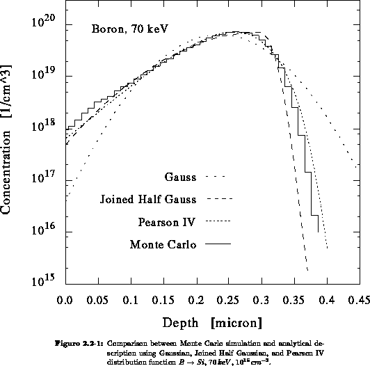
Figure 2.2-1 shows the comparison between Monte Carlo simulations and simulations using distribution functions. For all distribution functions (Gauss, Joined Half Gauss and Pearson IV) the same moments were used for calculating the parameters.
Recently, the application of a dual Pearson function (2.2-9),
has gained popularity in describing profiles with channeling tails
[Tas89], [Par90], [Gon92]. Two Pearson IV functions  and
and  are added up to give the actual profile. The parameter
  describes roughly the partition of the profile into an amorphous part and a
channeled part.
describes roughly the partition of the profile into an amorphous part and a
channeled part.
In other cases, where Pearson distributions do not agree well with measured profiles, they have been modified, e.g. by adding exponential tails [Hof75a], [Ant78]. Similar modifications are necessary for the description of damage profiles [Hob88b]. These manipulations are justified, since the only goal of analytical functions is to fit measurements or more sophisticated simulations.