


Next: 4. Quantum Confinement and
Up: 3.5 Strain and Bulk
Previous: 3.5.1 Deformation Potential Theory
Subsections
The k.p method allows to derive analytical expressions for the energy dispersion and the effective masses [161]. It enables the extrapolation of the band structure over the entire Brillouin zone from the energy gaps and matrix elements at the zone center. In addition to the common use of the k.p method to model the valence band of semiconductors, it is also well suited to describe the influence of strain on the conduction band minimum.
The k.p method can be derived from the one-electron Schrödinger equation as follows:
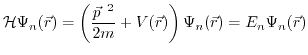 |
(3.26) |
 denotes the periodic lattice potential and
 the one-electron Hamilton operator.
  describes the one-electron wave function in an eigenstate
  and
and  the eigenenergy for the eigenstate . Due to the periodicity of the lattice potential (3.26) the Bloch theorem is applicable and the solution can be written in the form of:
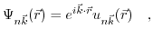 |
(3.27) |
The wave function
 can be expressed as the product of a plane wave and the function
 , which reflects the periodicity of the lattice. denotes the band index and
  represents a wave vector. If the given potential
only depends on one spatial coordinate (also called local), (3.27) can be substituted in (3.26).
represents a wave vector. If the given potential
only depends on one spatial coordinate (also called local), (3.27) can be substituted in (3.26).
Luttinger [173] showed that it is possible to use the eigenfunctions of the ground states as a complete set of eigenfunctions and that the wave function can be expanded by
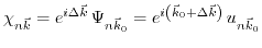 |
(3.28) |
for
 . Inserting (3.28) into (3.26) yields:
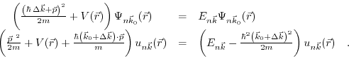 |
(3.29) |
This way, for any fixed wave vector
 , (3.29) for the unperturbed system, delivers a complete set of eigenfunctions
 , which completely cover the space of the lattice periodic functions in real space. Therefore, the wave function
at , for the full system, can be expressed via
, which completely cover the space of the lattice periodic functions in real space. Therefore, the wave function
at , for the full system, can be expressed via
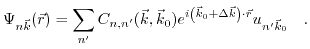 |
(3.30) |
As soon as the eigenenergy
 and the
of the unperturbed system are determined, the eigenfunctions
and eigenenergies
and the
of the unperturbed system are determined, the eigenfunctions
and eigenenergies
 can be calculated for any
 in the vicinity of
 by accounting the
 term in (3.29) as a perturbation. This method has been introduced by Seitz [174] and extended by [172,173,175] to study the band structure of semiconductors.
Due to the
term in (3.29) this method is also known as the k.p method. Provided that the energies at
and that the matrix elements of  between the wave functions, or the wave functions themselves, are known, the band structure for small
 's around
can be calculated. The entire first Brillouin zone can be calculated by diagonalizing (3.29) numerically, provided a sufficiently large set of
to approximate the complete set of basis functions is used [172].
's around
can be calculated. The entire first Brillouin zone can be calculated by diagonalizing (3.29) numerically, provided a sufficiently large set of
to approximate the complete set of basis functions is used [172].
The following subsections will explain the effective masses for the non-degenerate conduction band of silicon and the energy dispersion utilizing a non-degenerate k.p theory. In order to analyze the effects of shear strain on the two lowest conduction bands
 and
and
 , the k.p method is adapted to enable degeneracy, due to the coincidence of the
and
bands at the
, the k.p method is adapted to enable degeneracy, due to the coincidence of the
and
bands at the  point.
The conduction band minima of silicon reside on the
 axes at a distance of
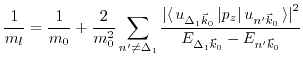
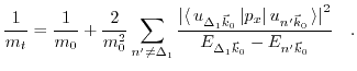
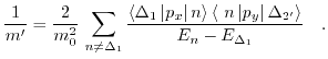
 from the symmetry points. By means of non-degenerate perturbation theory and the knowledge of the eigenenergies
and the wave functions
at the conduction band minima
, the eigenvalues
at neighboring points can be expanded to second order terms in
from the symmetry points. By means of non-degenerate perturbation theory and the knowledge of the eigenenergies
and the wave functions
at the conduction band minima
, the eigenvalues
at neighboring points can be expanded to second order terms in  .
.
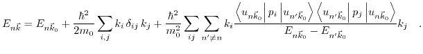 |
(3.31) |
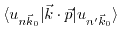
Scalar products
 are expressed via index notation
 and the matrix elements with Dirac's notation
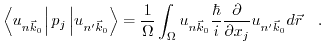 |
(3.32) |
The linear terms in can be set to zero under the assumption that
 is a minimum. The expression for the effective mass tensor
 can be derived from the dispersion relation (3.31)
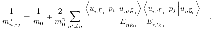 |
(3.33) |
The effective mass tensor for the lowest conduction band
in diamond crystal structures is characterized by two masses. In the principal coordinate system for the
![$ \left [001\right ]$](img8.png) valley the effective masses can be written as
valley the effective masses can be written as
 |
(3.34) |
and
 |
(3.35) |
denotes the band index of the lowest conduction band. Therefore, the energy dispersion can be formulated as:
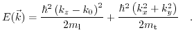 |
(3.36) |
From the derived equations follows that due to the coupling between electronic states in different bands (via k.p term), an electron in a solid has a different mass than a free electron. The coupling terms are related to the following criteria:
- The bigger the energetic gap between two bands, the smaller is the effect on the effective mass. The relative importance of a band
 to the effective mass of band is controlled by the energy gap between the two bands.
- All bands with non-zero matrix elements
 can be found via the matrix element theorem [176] by group theoretical considerations checking all possible symmetries for
 .
.
It is possible to calculate numerically all matrix elements and subsequently the effective masses from (3.33) via the empirical pseudo potential method [177].
(3.55) only requires the direction of the vector, indicating the location of the valley, to describe the shift of the valley minima. Hence, the valley shift is independent of the exact value of the wave vector and all points belonging to a particular valley experience the same shift. Since the effective mass is given by the second derivative of the energy dispersion
 and (3.16) does not change the curvature of the energy band, the formula predicts no change in the effective electron mass due to strain.
However, there is a clear experimental proof that shear strain changes the effective masses of electrons in the lowest conduction band[170] and the exciton spectrum of silicon[171]. In order to explain this behavior one has to take the splitting of the lowest two conduction bands at the symmetry point by shear strain into account. The lifting of the degeneracy can be calculated with the deformation potential constant  via (3.20). (3.20) is only valid at the symmetry point and cannot be used to predict the effect of strain on the valley minima
 . In order to circumvent this obstacle a degenerate k.p theory has to be applied around the symmetry point.
A different approach was adapted in [161]. The Hamiltonian at the
 points can be described via the theory of invariants:
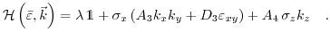 |
(3.37) |
where,
 |
(3.38) |
 and
and
 are the Pauli's matrices and
  and
and  denote scalar constants
 and and |
(3.39) |
The scalar constants  ,
,  , and
, and  are connected to the deformation potential constants
  ,
,  , and through
 |
(3.40) |
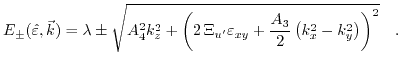
From (3.37) eigenvalues can be calculated which represent the energy dispersion for the first and second conduction band
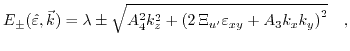 |
(3.41) |
where  denotes the energy dispersion of
and
denotes the energy dispersion of
and  that of
.
Under the assumption that this description is valid around the point up to the minimum of the lowest conduction band at
that of
.
Under the assumption that this description is valid around the point up to the minimum of the lowest conduction band at
 ,
,  and can be related to each other via
 |
(3.42) |
 describes the distance of the conduction band minimum of unstrained silicon to the point. can be determined from (3.42)
 |
(3.43) |
The effect of shear strain on the shape of the lowest conduction band is examined in the following section.
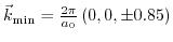
Up to now it has been assumed that the conduction band minima are located at
. This is only valid for small shear strain.
The minimum of the conduction band moves towards the point in conjunction with an increasing splitting between the conduction bands, when the shear strain rises (as can be seen in Fig. 3.2). This causes a change in the shape of the conduction bands and the assumption that the minima lie fixed at
does not hold anymore.
Therefore, a model which is able to cover the effects of shear strain on the effective masses has to take the movement of the conduction band as a function of strain into account. In the following a model will be derived that takes this movement of
 into account.
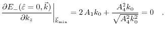
Starting with (3.41) and setting
 the minimum can be found from the dispersion relation
 |
(3.44) |
The constants and are replaced with the relations (3.43) and (3.36), and
 describes the position of the conduction band minimum measured from the zone boundary . Setting the first derivative of (3.44) to zero,
 , and solving for
  results in the desired relation between
 and shear strain.
 |
(3.45) |
Here
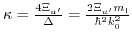 is introduced and represents the ratio between the shear deformation potential and the band separation between the two lowest conduction bands
  at zero shear strain (Fig. 3.3).
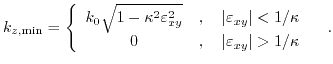
(3.45) shows that for strain smaller than
at zero shear strain (Fig. 3.3).
(3.45) shows that for strain smaller than  , the minimum position shifts towards the point. At
 , the minimum is located at the point (
 ). Increasing shear strain above
 does not shift
anymore. The change of shape of the two lowest conduction bands
and
and accordingly the position change of the minimum with increasing shear strain can be seen in Fig. 3.2.
does not shift
anymore. The change of shape of the two lowest conduction bands
and
and accordingly the position change of the minimum with increasing shear strain can be seen in Fig. 3.2.
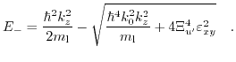
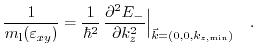
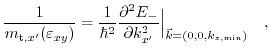
The strain dependent longitudinal mass
 can be calculated from (3.44) with
 |
(3.46) |
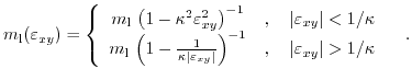
After some algebraic manipulations the strain dependent mass
can be expressed as
 |
(3.47) |
Accordingly to (3.45) the dependence of the longitudinal masses is different for a strain level above or below .
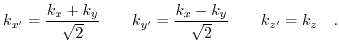
For the derivation of the transversal masses we rotate the principal coordinate system by
 around the z-axis with the following transformation:
 |
(3.48) |
The energy dispersion in the rotated coordinate system is
 |
(3.49) |
The effective mass in the
![$ \left[110\right]$](img403.png) and
and
![$ \left[ 1\bar{1}0\right]$](img522.png) directions is defined by
directions is defined by
 |
(3.50) |
and
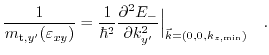 |
(3.51) |
Applying (3.50) and (3.51) to (3.49) gives for the
direction
 |
(3.52) |
and
 |
(3.53) |
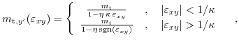
for the
direction with the parameter
 and
and  is defined by
 |
(3.54) |
As can be seen along the
direction the effective mass is reduced (mobility is enhanced) for
 , while for the
direction the effective mass is increased (the mobility is reduced) for increasing shear strain (
, while for the
direction the effective mass is increased (the mobility is reduced) for increasing shear strain (
 ). For shear strain above
the effective mass is a constant which depends on the sign of the strain.
). For shear strain above
the effective mass is a constant which depends on the sign of the strain.
The analytical valley shift induced by shear strain
 (given in (3.22)) can now be calculated. Substituting the expression for
from (3.45) into equation (3.44) delivers the equation for shear strain.The shift between the valley pair along
and the valley pairs
(given in (3.22)) can now be calculated. Substituting the expression for
from (3.45) into equation (3.44) delivers the equation for shear strain.The shift between the valley pair along
and the valley pairs
![$ \left [100\right ]$](img18.png) or
or
![$ \left [010\right ]$](img19.png) due to
can be obtained in the form of
due to
can be obtained in the form of
 |
(3.55) |
Next: 4. Quantum Confinement and
Up: 3.5 Strain and Bulk
Previous: 3.5.1 Deformation Potential Theory
T. Windbacher: Engineering Gate Stacks for Field-Effect Transistors