


Next: 4.4 Effective Mass of
Up: 4. Quantum Confinement and
Previous: 4.2 Effective Mass of
4.3 Quantization in UTB Films for Primed Subbands
As pointed out before a shear strain component in the
![$ \left[110\right]$](img403.png) direction does not affect the primed valleys along
direction does not affect the primed valleys along
![$ \left [100\right ]$](img18.png) and
and
![$ \left [010\right ]$](img19.png) direction, except for a small shift of the minimum [186]. However, the linear combination of bulk bands method gained with the empirical pseudo-potential calculations [4] and calculations of the primed subbands based on the density functional theory (DFT) [3] uncover the relationship of the transport effective masses on the silicon film thickness
direction, except for a small shift of the minimum [186]. However, the linear combination of bulk bands method gained with the empirical pseudo-potential calculations [4] and calculations of the primed subbands based on the density functional theory (DFT) [3] uncover the relationship of the transport effective masses on the silicon film thickness  .
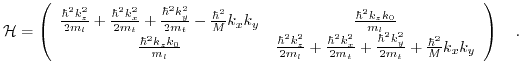
Here we analyze the dependence of the primed subbands effective mass via the two-band k.p Hamiltonian utilized before (4.1). At first we have to derive analogously to the unprimed subbands an analytical expression for
.
Here we analyze the dependence of the primed subbands effective mass via the two-band k.p Hamiltonian utilized before (4.1). At first we have to derive analogously to the unprimed subbands an analytical expression for  as a function of
  and vice versa:
 |
(4.27) |
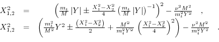
Starting with the transformation to dimensionless form according to:
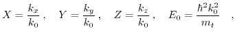 |
(4.28) |
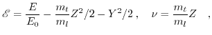
and some further rearrangements
 |
(4.29) |
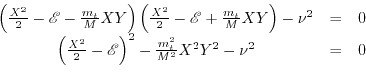
the eigenvalue problem takes the following form:
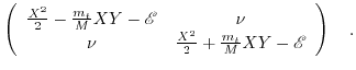 |
(4.30) |
Setting the determinant of (4.30) to zero allows to obatin  as a function of

 |
(4.31) |
Like before for the unprimed subbands, the obtained fourth order equation,
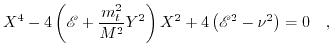 |
(4.32) |
can be reformulated into two second order equations:
 |
(4.33) |
The identities
 |
(4.34) |
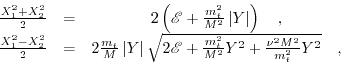
allow to introduce a
 dependence in (4.33) and formulate the problem as
 and vice versa
 |
(4.35) |
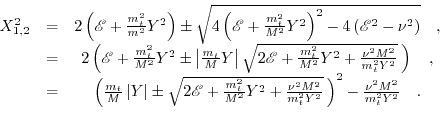
So  as a function of
  is described by the following equation:
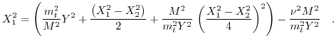 |
(4.36) |
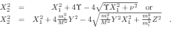
Substituting
 into (4.36) results in:
 |
(4.37) |
and enables the derivation of as a function of
 |
(4.38) |
In order to obtain
 the minus branch of (4.35) is used:
 |
(4.39) |
After analogous treatment of (4.39) the relation of as a function of is derived:
 |
(4.40) |
The corresponding scaled energy dispersion relation is given by:
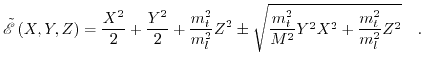 |
(4.41) |
Next: 4.4 Effective Mass of
Up: 4. Quantum Confinement and
Previous: 4.2 Effective Mass of
T. Windbacher: Engineering Gate Stacks for Field-Effect Transistors