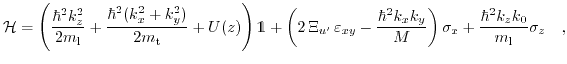
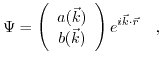
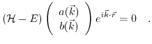
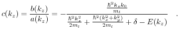
The two-band k.p Hamiltonian of a [001] valley in the vicinity of the X-point of the Brillouin zone in Si must be in the form [161]:
where
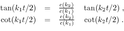
![]() are the Pauli matrices,
are the Pauli matrices,
![]() is the
is the ![]() unity matrix,
unity matrix,
![]() is the position of the valley minimum relative to the X-point in unstrained Si,
is the position of the valley minimum relative to the X-point in unstrained Si, ![]() with
with
![]() is the wave vector,
is the wave vector,
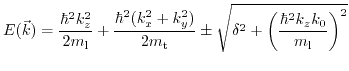
![]() denotes the shear strain component in physics notations,
denotes the shear strain component in physics notations,
![]() , and
, and
![]() is the shear strain deformation potential [161,170,179,180].
is the shear strain deformation potential [161,170,179,180].
![\includegraphics[width= 0.6\textwidth]{figures/drawing.ps}](img543.png)
|
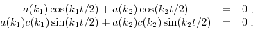
For a square well potential the wave function is set to zero at the boundaries, which allows an analytical analysis of the subband structure.
In the two-band model the wave function is a spinor with two components. Therefore, we use the following ansatz,
Taking the determinant of (4.3) and setting it to zero results in the energy dispersion relation of the system.
with
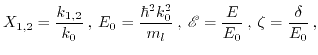
For each energy ![]() there are four solutions for
there are four solutions for ![]() . Fig. 4.2 shows that
. Fig. 4.2 shows that
![]() is even with respect to
is even with respect to ![]() . Therefore, there are always two independent values
. Therefore, there are always two independent values
![]() and
and
![]() for the wave vector, which are complemented to four values by alternating their signs.
For energies in the gap the two values are imaginary. The wave function is then a superposition of the solutions with the four eigenvectors:
for the wave vector, which are complemented to four values by alternating their signs.
For energies in the gap the two values are imaginary. The wave function is then a superposition of the solutions with the four eigenvectors:
 |
(4.6) |
![\includegraphics[width= 0.5\textwidth]{figures/Fig2.eps}](img555.png)
|
We introduce ![]() as the ratio between
as the ratio between ![]() and
and ![]() .
. ![]() is an odd function with respect to
is an odd function with respect to ![]() :
:
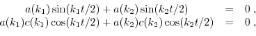
Additionally, fulfilling the boundary conditions
![]() demands that
demands that
![]() is satisfied.
Thus resulting in
is satisfied.
Thus resulting in
 |
(4.8) |
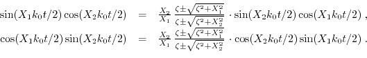
Expressing ![]() with (4.9) and putting them into (4.10) leads to these two conditions:
with (4.9) and putting them into (4.10) leads to these two conditions:
 |
(4.11) |
 |
(4.12) |
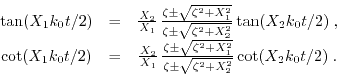
and a few calculation steps found in the Appendix A., the equations can be written in the form:
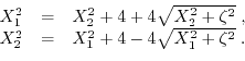
For the numerical solution it is convenient to reformulate the equations as:
![]() and
and ![]() coexist in the equations. Therefore, we need an extra relation to re-express
coexist in the equations. Therefore, we need an extra relation to re-express ![]() as a function of
as a function of ![]() or vice versa, the derivation of which can be found in the Appendix A.:
or vice versa, the derivation of which can be found in the Appendix A.:
Eliminating one of the two ![]() 's with (4.15) in (4.14) allows to calculate
's with (4.15) in (4.14) allows to calculate ![]() as a function of strain
as a function of strain ![]() . Then one can calculate the energy as a function of strain
. Then one can calculate the energy as a function of strain ![]() by using (4.4).
by using (4.4).
![\includegraphics[width= 0.5\textwidth]{figures/Fig3b.eps}](img571.png)
|
Interestingly, (4.13) coincides with the dispersion relations obtained from an auxiliary tight-binding consideration [181]. For ![]() (4.13) become equivalent.
For higher strain values (4.14) must be solved numerically.
The value
(4.13) become equivalent.
For higher strain values (4.14) must be solved numerically.
The value
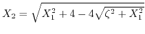 becomes imaginary at high strain values. In this case the trigonometric functions in (4.13) or (4.14) are replaced by the hyperbolic ones. Special care must be taken to choose the correct branch of
![]() in (4.13) or alternatively (4.14). The sign of
in (4.13) or alternatively (4.14). The sign of
![]() must be alternated after it becomes zero, as it is displayed in Fig. 4.3.
must be alternated after it becomes zero, as it is displayed in Fig. 4.3.
![\includegraphics[width= 0.6\textwidth]{figures/Fig4.eps}](img576.png)
|
![\includegraphics[width= 0.6\textwidth]{figures/Fig5.eps}](img578.png)
|
![\includegraphics[width= 0.6\textwidth]{figures/Fig6.eps}](img579.png)
|
Fig. 4.4 and Fig. 4.5 show the energies of the subbands as a function of shear strain for two different film thicknesses. Shear strain opens the gap between the two conduction bands at the X-point making the energy dispersion non-parabolic [179], which removes the subband degeneracy and introduces the valley splitting. Fig. 4.6 and Fig. 4.7 show the energy difference between two unprimed subbands
![]() as a function of strain for the same quantum number
as a function of strain for the same quantum number ![]() .
.
![\includegraphics[width= 0.6\textwidth]{figures/Fig7.eps}](img580.png)