3.4.2 Oct-Tree

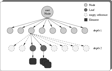
An oct-tree is a data structure to perform three-dimensional point locations and range searches. In a finite oct-tree the geometrical data are presorted in a way that allows efficient element searches. The space containing a grid is recursively decomposed into $8$ sub-spaces. A sub-space can either be a node or a terminal leaf. A node is an intermediate sub-space that does not contain any elements itself but serves as a container for other sub-nodes or sub-leafs. A terminal leaf represents a situation where a further split would not reduce the number of elements in at least one of the resulting sub-leafs (Fig. 3.12).

Figure 3.12: Node/leaf hierarchy of an oct-tree.

The effort to search for an element in an oct-tree is of order $O(\log{n})$ which gives the best possible performance among the two point location methods presented in this thesis. This nearly optimal search performance is due to the drastic recursive decomposition of space in $8$ sub-spaces respectively. For homogeneous grid density, every search step reduces the remaining elements to search by a factor of $8$.

The major disadvantages of a finite oct-tree are time consuming pre-processing and memory overheads. The pre-processing time is related to the algorithm that inserts elements into the oct-tree. For every grid element it must be decided to which (already existing) sub-node it belongs. This results in a large number of geometrical predicates that have to be computed until the final sub-space, the so-called terminal leaf, is found. Furthermore, if a grid element collides with a terminal leaf, this leaf must be replaced by a node and all elements of that leaf have to be re-distributed over the newly created sub-spaces. Depending on how the elements are shaped and how they fit into already existing leafs the complexity of such a test can vary significantly. In case one of the points is contained within a leaf the test is reduced to a simple point compare operation. In the worst case the orientation of several tetrahedrons has to be computed. Every inserted element traverses all nodes until it reaches the terminal leaf. On every node level all sub-spaces that overlap the element must be computed. For each overlapping sub-space the algorithm recurses into the node or leaf associated to the sub-space. For a homogeneous grid the majority of grid elements will only overlap one sub-node in any given level. Thus the amount of overlap decisions per element can be estimated to $8\cdot D$ where $D$ is the depth of the oct-tree.

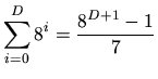
Obviously the memory overhead results from the nodes and terminal leafs that hold the data. For an average depth $D$ of the oct-tree the number of nodes and leafs results to:

$$\sum_{i=0}^{D}{8^i} = \frac{8^{D+1}-1}{7}$$ (3.1)

To give an example lets compute the memory consumption including the overhead to store a number of $N=2\cdot10^6$ homogeneously distributed tetrahedrons on a $32$ bit machine. The average depth $D$ is given as $log_{8}N \approx 7$. According to (3.1) the number of nodes and leafs computes to $\approx 2.4\cdot10^6$. This is of the same magnitude as the number of elements that are stored. A tetrahedron as it is stored in the oct-tree consists of $4$ point references (handles, c. f. Chapter 3.7.1), thus the per tetrahedron memory consumption is $32$ bytes. If we estimate an average of $6$ tetrahedrons that share a point we have a total of $\approx 5\cdot10^5$ points in our example. A point coordinate is stored as an IEEE754 double precision floating point number that takes $8$ bytes. The memory needed to store the data is then $2.4\cdot10^6\cdot32\approx77$ megabytes for the tetrahedrons and $5\cdot10^5\cdot24=12$ megabytes for the points, which gives a total of $\approx 89$ megabytes.

A node consists of $8$ references to sub-nodes or leafs and two references to points, which amounts to $80$ bytes of memory. The last of the $7$ layers in the oct-tree structure always consists of leafs, thus the total number of nodes in our example is $\approx 3\cdot 10^5$ which gives a memory consumption of $\approx 24$ megabytes. For the remaining leafs ( $\approx 2\cdot 10^6$) the memory consumption depends on the type of the leaf. Every leaf stores two point references. Additionally, the smallest leaf stores a reference to one element, the largest holds an arbitrary number of references. To make a guess we assume that the medium number of stored element references is three. The average memory consumption per leaf is then $5\cdot 8=40$ bytes and the total amount of memory for the leafs is $\approx 80$ megabytes. The total of the introduced memory overhead in this example amounts to $104$ megabytes. If we relate the memory for the data to the introduced overhead it gives $\approx 110\%$. The number of overlap tests is also quite impressive, it can be estimated to be in the order of $\approx 10^8$.

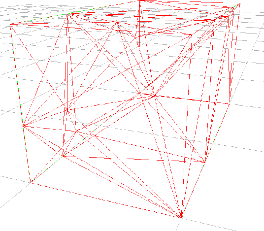
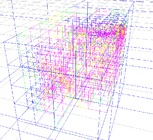
A finite oct-tree that implements the decomposition algorithm was developed at the Institute for Microelectronics [28]. The methods used to determine whether an element overlaps a leaf are encapsulated in an interface. This allows arbitrary elements to be governed by the oct-tree as long as they implement this interface. Fig. 3.13 and Fig. 3.14 depict a small mesh and the resulting leaf structure in the finite oct-tree.

Figure 3.13: Cuboidal region.

Figure 3.14: Resulting leaf structure for cuboidal region.

There is also a parallelized version of this algorithm [47,48] available that distributes sub-trees over various networked computers to utilize several CPUs. For communication between the computers the high-level protocol CORBA [49] was used. CORBA is a standard that allows to call methods of remote objects. The location of the object is thereby transparent to the client. The connection between client and remote (server) object is established via an object reference. The references of objects are managed by the CORBA nameserver. The client contacts the nameserver upon startup and requests a reference to a certain object. Such a high-level protocol imposes a considerable overhead compared to a local function call. The overhead is observed as a time delay or as a maximum number of method invocations per second. The delay is closely related to speed and workload of the underlying network infrastructure.

The efficiency of the parallelization is determined by the time delay and the remote CPU time that is consumed by the remote method. If the relation between delay and CPU time is low, or -- in other words -- if a complex remote computation takes place, then the overhead can be neglected. This is the case for the fairly time consuming oct-tree insert method. During the implementation it turned out, however, that the serialization and dynamic instantiation of objects that is necessary to transfer an object (like, e.g. a point) over the network is not well supported in the target language (C++) and imposes an extra programming overhead for each element type. This is in the contrary to the design of the single-threaded oct-tree which is capable of storing arbitrary elements without the need to recompile the oct-tree source code.

Future developments will focus on a multi-threaded version of the oct-tree where only CPUs on one machine can be utilized.

The decision whether an application uses the oct-tree or rather the jump-and-walk algorithm presented in the next section strongly depends on the amount of point locations that will be performed during the simulation. Fig. 3.13 and Fig. 3.14 show a grid of a cuboidal region and the resulting sub-division into nodes and leafs.

2003-03-27