Next: 4.4 Bulk Mobility of
Up: 4. Mobility Modeling
Previous: 4.2 Modeling Approaches
Subsections
4.3 Bulk Mobility of Strained Si
For low values of the electric fields, the carriers are almost in equilibrium
with the lattice vibrations and the low-field mobility is mainly affected by
phonon and Coulomb scattering. For device simulation purposes, several mobility
models have been suggested for unstrained Si which are mostly semi-empirical
in nature. Established models are due to Caughey and Thomas
[Caughey67], Arora [Arora82], and Klaassen [Klaassen92]
who suggested a unified low-field mobility model.
As was discussed in Section 3.3.3, the presence of mechanical
strain modifies the relative position of the different valleys in the
conduction band. A first order estimate of these effects on the mobility can be
obtained using the piezoresistance model.
4.3.1 Piezoresistance Model
Piezoresistivity is the phenomena referring to the coupling between electrical
conductivity (resistivity) and mechanical stress. Fig. (4.2) shows
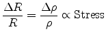
how the resistance of a n-type Si sample varies with hydrostatic stress. The
resistance decreases linearly with stress until 20GPa. This change in
resistance is related to a change in the resistivity,  and can be
expressed as
and can be
expressed as
 |
(4.33) |
Figure 4.2:
Resistance of n-type Si sample as a function of the hydrostatic
pressure. Figure adapted from [Seeger88](Fig.4.26).
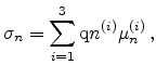
The variation of the mobility with applied stress can be obtained from the
piezoresistive coefficients originally measured by Smith [Smith54]. In the
presence of stress, the conductivity of the unstrained semiconductor,
 |
(4.34) |
gets modified to
 |
(4.35) |
Here  and
and
 denote respectively, the carrier
concentration and mobility in the
denote respectively, the carrier
concentration and mobility in the  valley pair in strained Si. Assuming
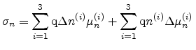
a doped semiconductor, (
valley pair in strained Si. Assuming
a doped semiconductor, (
 ), the change in conductivity is given
as [Manku93a].
), the change in conductivity is given
as [Manku93a].
 |
(4.36) |
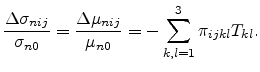
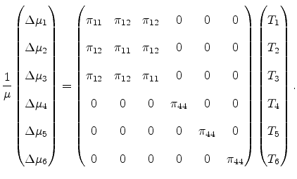
Here  are the components of the strain tensor. The quantity
 is a fourth rank tensor of piezoresistance coefficients which are
a measure of the first order change in normalized resistivity per unit applied
stress for different stress directions. It has 81 elements which upon the
application of the point group symmetry operations reduces to only 3
piezoresistance coefficients,
is a fourth rank tensor of piezoresistance coefficients which are
a measure of the first order change in normalized resistivity per unit applied
stress for different stress directions. It has 81 elements which upon the
application of the point group symmetry operations reduces to only 3
piezoresistance coefficients,  ,
, and
and
 . Table 4.3.1 lists the values of these
piezoresistance coefficients for n-type and p-type Si. Using the contracted
notation shown in (3.16), the change in mobility can be
expressed as
. Table 4.3.1 lists the values of these
piezoresistance coefficients for n-type and p-type Si. Using the contracted
notation shown in (3.16), the change in mobility can be
expressed as
Table 4.1:
Measured values of piezoresistance coefficients taken from Smith [Smith54]
 |
(4.37) |
4.3.2 Physically Based Mobility Model for Strained Si
To develop an electron mobility model for Si under different strain conditions,
the relative electron population of the different valleys in Si have to be
properly considered [Manku92,Egley93].
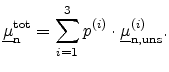
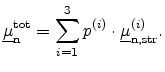
As suggested in [Manku92], the anisotropic electron mobility in strained
Si can be computed as the weighted average of the unstrained electron mobility
tensor,
 , of the conduction band valley
pair in Si with the corresponding electron population,
, of the conduction band valley
pair in Si with the corresponding electron population,  in the
pair,
in the
pair,
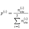
The relative populations of each valley pair is given by
where
 is calculated for non-degenerate doping concentrations
using Boltzmann statistics with
is calculated for non-degenerate doping concentrations
using Boltzmann statistics with
 as the effective density of
states.
as the effective density of
states.
The
 denote the strain-induced energy shifts which can
be computed from deformation potential theory discussed in
Section 3.3.1.1. The
denote the strain-induced energy shifts which can
be computed from deformation potential theory discussed in
Section 3.3.1.1. The
 refer to the
unstrained electron mobilities in the valley pair.
refer to the
unstrained electron mobilities in the valley pair.
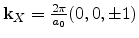
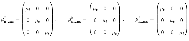
Here  and
and  denote the mobilities along the major and minor axes
in each ellipsoid, respectively. The
denote the mobilities along the major and minor axes
in each ellipsoid, respectively. The
 denote the
electron mobility tensors for Si for the [100], [010], and [001] valley pairs
corresponding to directions
denote the
electron mobility tensors for Si for the [100], [010], and [001] valley pairs
corresponding to directions  ,
,  , and
, and  , respectively. Using
(4.38) to (4.41), the in-plane (x-component) and
perpendicular components (z-component) of the electron mobility in strained Si
on a (001) SiGe substrate can be expressed as
, respectively. Using
(4.38) to (4.41), the in-plane (x-component) and
perpendicular components (z-component) of the electron mobility in strained Si
on a (001) SiGe substrate can be expressed as
In arriving at (4.42) and (4.43), the relation
 has been used which is a consequence of the biaxial
tensile strain resulting from growing Si on SiGe (see
Section 3.3.3.1). The unstrained mobility can be obtained by
setting
has been used which is a consequence of the biaxial
tensile strain resulting from growing Si on SiGe (see
Section 3.3.3.1). The unstrained mobility can be obtained by
setting
 .
.
Figure 4.3:
In-plane and perpendicular electron mobilities in undoped strained Si
versus the Ge content in the [001] oriented SiGe buffer layer calculated
using (4.42) and (4.43). Also shown is the mobility
obtained from piezoresistance coefficients [Smith54] [Kanda82] as
described in Section 4.3.1 and from Monte Carlo
simulations.
Equations (4.42) and (4.43) represent the
model in [Manku92]. The resulting in-plane and out-of-plane electron
mobilities in a strained Si layer as a function of the Ge content in the
SiGe (001) substrate is shown in Fig. 4.3. The model reproduces the
linear increase (decrease) in the in-plane (out-of-plane) electron mobility
component for low strain followed by mobility saturation for high strain
levels. However, the model shows a too high value of the unstrained mobility if
the saturation mobility values are fixed. This is due to the fact that it does
not consider the effect of inter-valley scattering which is present in
unstrained Si and results in a lower mobility. The model in (4.42)
and (4.43) uses only the two parameters, and , with
which it is not possible to match three quantities simultaneously such as the
unstrained, and the strained in-plane and perpendicular electron
mobilities.
To improve the electron mobility model for strained Si, the effect of
inter-valley scattering is included. Equation (4.38) is modified as
follows
Here the
 denote the electron mobility tensors of
strained Si for the [100], [010], and [001] valleys pairs. In (4.45) a
mobility tensor is modeled as a product of a scalar mobility and the scaled
inverse mass tensor.
denote the electron mobility tensors of
strained Si for the [100], [010], and [001] valleys pairs. In (4.45) a
mobility tensor is modeled as a product of a scalar mobility and the scaled
inverse mass tensor.
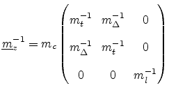
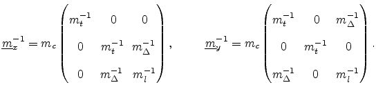
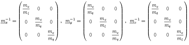
The scaled inverse effective mass tensors for the , and directions
are given as
with  and
and  denoting the transversal and longitudinal masses,
respectively for the ellipsoidal
denoting the transversal and longitudinal masses,
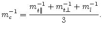
respectively for the ellipsoidal  -valleys in Si. The mass tensors are
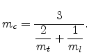
scaled to a dimensionless form by the conductivity mass
-valleys in Si. The mass tensors are
scaled to a dimensionless form by the conductivity mass 
From this scaling it follows that
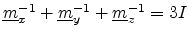 , where
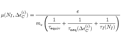
  denotes the identity matrix. The scalar mobility
 includes the dependences on the energy shifts
 and
the doping concentration
and
the doping concentration  of the strained Si layer.
In (4.49) the following momentum relaxation times are assumed:
-
 for acoustic intra-valley scattering and inter-valley scattering between equivalent valleys (
 -type).
-
 for inter-valley scattering between non-equivalent valleys (
 -type scattering).
-
 for impurity scattering.
Figure 4.4:
Inter and intra valley transitions within the 3 valley pairs in
Si.
Fig. ![[*]](crossref.png) illustrates the f-type and g-type scattering
mechanisms. The effect of the different scattering mechanisms on the total
mobility is estimated by Matthiessen's rule, see (4.49). To arrive at a
formal description of the mobility components in strained Si in terms of
measurable macroscopic quantities, the following cases are considered.
illustrates the f-type and g-type scattering
mechanisms. The effect of the different scattering mechanisms on the total
mobility is estimated by Matthiessen's rule, see (4.49). To arrive at a
formal description of the mobility components in strained Si in terms of
measurable macroscopic quantities, the following cases are considered.
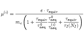
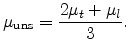
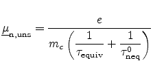
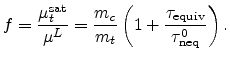
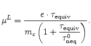
The scalar electron mobility for unstrained and undoped Si, also referred to as
lattice mobility  , can be derived by dropping the impurity scattering
rate in (4.49).
, can be derived by dropping the impurity scattering
rate in (4.49).
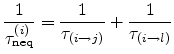
Here
 denotes the inter-valley relaxation time for -type phonon
scattering in unstrained Si. Since in the unstrained case all three valley
pairs are equally populated, we have
denotes the inter-valley relaxation time for -type phonon
scattering in unstrained Si. Since in the unstrained case all three valley
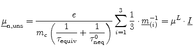
pairs are equally populated, we have
 . Using (4.49) the total unstrained mobility can then be written as
Note that the sum evaluates to the identity matrix
 .
.
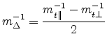
When dealing with in-plane biaxial tensile strain, the 6-fold degenerate
 -valleys in Si are split into 2-fold degenerate
  valleys
(lower in energy) and 4-fold degenerate
valleys
(lower in energy) and 4-fold degenerate  valleys (higher in energy)
with electrons preferentially occupying the lower energy levels. Under such
conditions, the electron mobilities in the in-plane and perpendicular
directions saturate. The saturation values can be obtained from (4.45)
by setting
valleys (higher in energy)
with electrons preferentially occupying the lower energy levels. Under such
conditions, the electron mobilities in the in-plane and perpendicular
directions saturate. The saturation values can be obtained from (4.45)
by setting
 .
.
Here it is assumed that the strain-induced valley splitting is large enough
such that the lowest valley is fully populated and the inter-valley scattering
to higher valleys is suppressed.
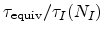
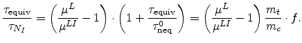
The ratio of the fully-strained mobility
 to the
unstrained mobility
to the
unstrained mobility  defines the mobility enhancement factor
In analogy with (4.49) the electron mobility for unstrained Si with
doping concentration can be written as
where
 signifies the lattice mobility including the effect of
impurity scattering. Multiplying the RHS of (4.54) with
signifies the lattice mobility including the effect of
impurity scattering. Multiplying the RHS of (4.54) with
 gives
gives
Rearranging (4.55), we can express the ratio
 as
as
From (4.51), the lattice mobility can be rewritten as
Substituting the value of
 from (4.57) into (4.56) gives
The last relation in (4.58) is obtained using (4.53).
The inter-valley scattering rate is a function of the strain-induced splitting
of the valleys. It can be expressed by using a dimensionless factor  ,
such that
,
such that
In strained Si, the total rate for electrons to scatter from initial valley  to final valleys
  and
and  is given by
 |
(4.60) |
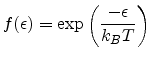
For low electric fields an equilibrium distribution function can be assumed and
 can be calculated [Conwell67]:
with the inter-valley scattering rate  defined as
and the Boltzmann distribution function
 .
.
 |
(4.65) |
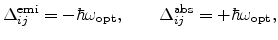
Here
 denotes the phonon energy and
the strain induced splitting, and C is a constant. A
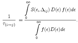
more accurate formalism for calculating the scattering rate would be through
the incorporation of the density of states
denotes the phonon energy and
the strain induced splitting, and C is a constant. A
more accurate formalism for calculating the scattering rate would be through
the incorporation of the density of states
 into (4.61),
giving [Seeger88]
into (4.61),
giving [Seeger88]
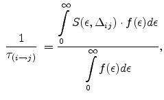
The calculation of the scattering rate using (4.61) and (4.66)
is shown in Appendix A. For our modeling purpose, the definition
in (4.61) leading to simpler expressions was found to be sufficient.
Using these expressions,
 can be expressed as
The function is defined as
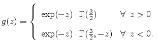 |
(4.68) |
Here
 and
and
 denotes the incomplete Gamma function. In the
unstrained case
denotes the incomplete Gamma function. In the
unstrained case
 |
(4.69) |
and therefore the unstrained inter-valley relaxation time
 can
be obtained as
can
be obtained as
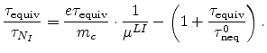
The factor in (4.59) is thus determined from (4.67)
and (4.70).
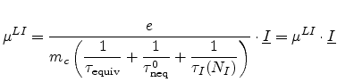
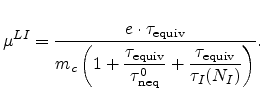
Multiplying the RHS of (4.49) with
gives
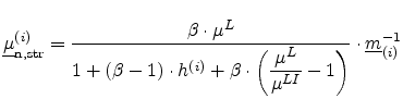
Using the relations in (4.53), (4.57) and (4.58), the
electron mobility for the valley in strained Si can be written as
where
 denotes the scaled effective mass tensor for the
valley pair in (4.47) and
denotes the scaled effective mass tensor for the
valley pair in (4.47) and
 . Equation (4.72) is plugged into (4.45) to
give the total mobility tensor for electrons in strained Si as a function of
doping concentration and strain. The tensor in (4.72) is given
in the principal coordinate system and has diagonal form.
. Equation (4.72) is plugged into (4.45) to
give the total mobility tensor for electrons in strained Si as a function of
doping concentration and strain. The tensor in (4.72) is given
in the principal coordinate system and has diagonal form.
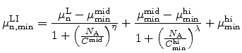
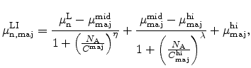
4.3.3 Doping Dependence
The doping and strain dependence of the in-plane and perpendicular electron
mobilities in Si is calculated using (4.72) by adopting any suitable
expression describing the doping dependence in unstrained Si. A model
distinguishing between the doping dependence,
 of the majority and
minority electrons in
of the majority and
minority electrons in
 has been suggested
in [Palankovski04,Kosina98]
has been suggested
in [Palankovski04,Kosina98]
 |
(4.73) |
 |
(4.74) |
where,
 is the mobility for the undoped material,
 is
the mobility at the highest doping. All other parameters are used as fitting
parameters. Although initially proposed for the majority electron mobility in
Si, equation (4.74) offers enough flexibility to model also
the minority electron mobility in Si. The difference between majority and
minority electron mobilities [Masetti83] is caused by effects such as
degeneracy and the different screening behavior of electrons and holes in the
semiconductor. Equation (4.74) describes a mathematical
function with two extreme values and can deliver a second maximum or minimum at
very high doping concentrations depending on the sign of
is
the mobility at the highest doping. All other parameters are used as fitting
parameters. Although initially proposed for the majority electron mobility in
Si, equation (4.74) offers enough flexibility to model also
the minority electron mobility in Si. The difference between majority and
minority electron mobilities [Masetti83] is caused by effects such as
degeneracy and the different screening behavior of electrons and holes in the
semiconductor. Equation (4.74) describes a mathematical
function with two extreme values and can deliver a second maximum or minimum at
very high doping concentrations depending on the sign of  . Thus, it
allows both majority and minority carrier mobilities to be properly
modeled.
. Thus, it
allows both majority and minority carrier mobilities to be properly
modeled.
The effect of shear stress on the band structure was discussed in
Section 3.3.4. For tensile stress along [110] the
energy dispersion of the lowest conduction band is influenced as follows:
- The valleys located along the
![$ [100]$](img207.png) and
and ![$ [010]$](img255.png) directions
move up in energy with respect to the valleys located along the
directions
move up in energy with respect to the valleys located along the
![$ [001]$](img256.png) direction.
direction.
- The shape of the valleys located along the direction is distorted
which results in a variation of the effective masses.
- The band minima of the valley pair along the direction
move towards the zone boundary
 points,
 .
.
The model presented in Section 4.3.2 relies on a) a model for the
momentum relaxation time, b) the relative populations of the different valley
pairs as a result of the energy shifts, and c) an effective mass tensor (with
constant  and
and  ), which basically provides the tensorial description
to the mobility. However, as discussed in
Section 3.3.4, in the presence of a uniaxial tensile
stress along
), which basically provides the tensorial description
to the mobility. However, as discussed in
Section 3.3.4, in the presence of a uniaxial tensile
stress along
 the two-fold degenerate -valleys
which are lowered in energy experience a change in the effective masses.
the two-fold degenerate -valleys
which are lowered in energy experience a change in the effective masses.
For the calculation of the mobilities in the presence of shear strain, the
effective mass tensors in (4.47) have to be modified.
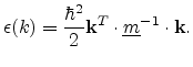
Using (3.35) the energy dispersion relation for the lower lying
valleys for stress along the ![$ [110]$](img208.png) direction can be rewritten as
direction can be rewritten as
![$\displaystyle \epsilon({\mathbf{k}}) = \frac{\hbar^2}{2}\left( \frac{k_{[110]}^...
...ert}} + \frac{k_{[\overline{1}10]}^2} {m_{t\perp}} + \frac{k_z^2}{m_l}. \right)$](img596.png) |
(4.75) |
Utilizing the transformation (3.66), the dispersion relation in
the principal coordinate system ( ) modifies to
![$\displaystyle \epsilon({\mathbf{k}}) = \frac{\hbar^2}{2}\left( k_x^2\left[\frac...
...rac{1}{m_{t\vert\vert}}-\frac{1}{m_{t\perp}}\right] + \frac{k_z^2}{m_l} \right)$](img598.png) |
(4.76) |
which can be expressed as
Here
 and the matrix
 denotes the
inverse mass tensor,
denotes the
inverse mass tensor,
The transversal masses along the and
![$ [\overline{1}10]$](img605.png) directions of
the -valleys are defined by
directions of
the -valleys are defined by
 and
and
 ,
respectively. The variation of these masses can be expressed as a function of
strain as described in (3.73)
and (3.74). Substituting (4.78) into (4.72)
gives the mobility tensor which now has a non-diagonal form in the principal coordinate system.
,
respectively. The variation of these masses can be expressed as a function of
strain as described in (3.73)
and (3.74). Substituting (4.78) into (4.72)
gives the mobility tensor which now has a non-diagonal form in the principal coordinate system.
The scaled inverse mass tensor in (4.78) was derived assuming only
 to be non-zero. For non zero values of the
 and
and
 shear strain components, the scaled inverse mass tensor
in (4.78) can be permutated to obtain the scaled inverse mass
tensors for the and valleys as
shear strain components, the scaled inverse mass tensor
in (4.78) can be permutated to obtain the scaled inverse mass
tensors for the and valleys as
 |
(4.82) |
Next: 4.4 Bulk Mobility of
Up: 4. Mobility Modeling
Previous: 4.2 Modeling Approaches
S. Dhar: Analytical Mobility Modeling for Strained Silicon-Based Devices
![\includegraphics[width=2.3in,angle=0]{figures/SeegerFig426_1.eps}](img484.png)
![\includegraphics[width=3in]{figures/rot_plot_manku_orig_review.eps}](img523.png)
![\includegraphics[width=2.2in,angle=0]{figures/Si_inter_intra.eps}](img542.png)
![$\displaystyle S(\epsilon,\Delta_{ij}) =C\cdot \left[(\epsilon - \Delta_{ij}^{\t...
...{\text{opt}}}{k_{B}T}\right)(\epsilon - \Delta_{ij}^{\text{abs}})^{1/2} \right]$](img567.png)
![$\displaystyle n_\ensuremath{{\mathrm{str}}}^{(i)} = N_C^{(i)} \cdot\exp \left[\frac{\Delta{\epsilon _C^{(i)}} }{ k_{B}T }\right]$](img510.png)
![$\displaystyle \mu_{\parallel} = \frac{ (\mu_l + \mu_t)\exp{[-\Delta \epsilon ^x...
...BT)]} }{2\exp{[-\Delta \epsilon ^x/(k_BT)]+\exp{[-\Delta \epsilon ^z/(k_BT)]}}}$](img518.png)
![$\displaystyle \mu_{\perp} = \frac{ 2\mu_t \exp{[-\Delta \epsilon ^x/(k_BT)]} + ...
...BT)]} }{2\exp{[-\Delta \epsilon ^x/(k_BT)]+\exp{[-\Delta \epsilon ^z/(k_BT)]}}}$](img519.png)

![$\displaystyle \frac{1}{\tau_{\text{neq}}^{(i)}} = C \left[ g\left(\displaysty...
...(\displaystyle \frac{ \Delta_{ij}^{\text{abs}}}{k_{B}T}\right)\right ] \right].$](img575.png)
![$\displaystyle \frac{1}{\tau_{\text{neq}}^{0}} = 2 C \left[g\left(\displaysty...
...{opt}}} {k_{B}T}\right) + \displaystyle \Gamma\left(\frac{3}{2}\right) \right].$](img581.png)