2.3.3.3 Drift-Diffusion Transport Model - Closure at $\phi _2$

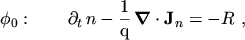
By taking only the first two moments, eqns. (2.99) and (2.102), into account

$$\phi_0: \textcolor{lightgrey}{.......}\ensuremath{\partial_{t} \,... ...rm{\nabla}}}}\ensuremath{\cdot}\ensuremath{\boldsymbol{\mathrm{J}}}_n}= - R \ ,$$ (2.141)

$$\ensuremath{\boldsymbol{\mathrm{\phi}}}_1: \textcolor{lightgrey}{... ...i_2 \rangle}}+ \mathrm{q}\, \ensuremath{\boldsymbol{\mathrm{E}}}\, n \Bigr) \ ,$$ (2.142)

and closing the equation system at $\phi _2$

$$\ensuremath{\langle \phi_2 \rangle}= \frac{3}{2} \, \mathrm{k}_\mathrm{B}\, n \, T_\mathrm{L}\ ,$$ (2.143)

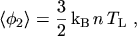
the drift-diffusion transport model is obtained. Since no information about the carrier temperature is available, the carrier temperature is set equal to the lattice temperature $T_n \equiv T_\mathrm{L}$, assuming the thermal equilibrium approximation [31].

$$\ensuremath{\ensuremath{\ensuremath{\boldsymbol{\mathrm{\nabla}}}}\ensuremath{\cdot}\ensuremath{\boldsymbol{\mathrm{J}}}_n} = \mathrm{q}\, (R + \ensuremath{\partial_{t} \, n}) \ ,$$ (2.144)

$$\ensuremath{\boldsymbol{\mathrm{J}}}_n = \mu_n \, \mathrm{k}_\mathrm{B}\, \Bigl( \ensuremath{\ensuremath... ...}{\mathrm{k}_\mathrm{B}} \, \ensuremath{\boldsymbol{\mathrm{E}}}\, n \Bigr) \ .$$ (2.145)

This transport model takes only local quantities into account. As such, it completely neglects non-static transport effects which occur in response to a sudden variation of the electric field, either in time or in space.

In order to enhance the validity range of the drift current expression, a field dependent mobility^2.10 is generally used, accounting for hot-carrier effects. Diffusivity, however, is largely underestimated with the EINSTEIN equations, if the lattice temperature rather than the carrier temperature is being used [7, p.145].

If needed, the average energy can be estimated via the homogeneous energy balance equation

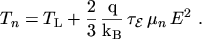$$T_n = T_\mathrm{L}+ \frac{2}{3} \, \frac{\mathrm{q}}{\mathrm{k}_\mathrm{B}} \, \tau_\mathcal{E}\, \mu_n \, E^2 \ .$$ (2.146)

However, for rapid increasing electric fields, for instance, the average energy lags behind the electric field. As a consequence the average energy can be considerably smaller than the one predicted by the homogeneous energy balance equation (2.146). Another important consequence is that the lag of the average energy gives rise to an overshoot in the carrier velocity. The reason for this velocity overshoot is that the mobility depends to first order on the average energy rather than on the electric field. As the mobility has not yet been reduced by the increasing energy but the electric field is already high, an overshoot in the velocity $\ensuremath{\boldsymbol{\mathrm{v}}} = \mu \, \ensuremath{\boldsymbol{\mathrm{E}}}$ is observed until the carrier energy comes into equilibrium with the electric field again. One of the first works dealing with this effect is [35]. Non-local effects like this one cannot be modeled using the drift-diffusion transport model.

M. Gritsch: Numerical Modeling of Silicon-on-Insulator MOSFETs PDF