2.3.3.5 Six Moments Transport Model - Closure at $ \phi _6$

Taking the first six moments, eqns. (2.99) to (2.104), into account give three balance and three flux equations

  $\displaystyle \phi_0:$ $\displaystyle \textcolor{lightgrey}{.......}$ $\displaystyle \ensuremath{\partial_{t} \, n}$   $\displaystyle - \frac{1}{\mathrm{q}} \, \ensuremath{\ensuremath{\ensuremath{\bo...
...bol{\mathrm{\nabla}}}}\ensuremath{\cdot}\ensuremath{\boldsymbol{\mathrm{J}}}_n}$       $\displaystyle = - R \ ,$ (2.168)
  $\displaystyle \phi_2:$ $\displaystyle \textcolor{lightgrey}{.......}$ $\displaystyle \frac{3}{2} \, \mathrm{k}_\mathrm{B}\, \ensuremath{\partial_{t} \, (n \, T_n)}$   $\displaystyle + \ensuremath{\ensuremath{\ensuremath{\boldsymbol{\mathrm{\nabla}}}}\ensuremath{\cdot}\ensuremath{\boldsymbol{\mathrm{S}}}_n}$   $\displaystyle - \ensuremath{\boldsymbol{\mathrm{E}}}\ensuremath{\cdot}\ensuremath{\boldsymbol{\mathrm{J}}}_n$   $\displaystyle = - \frac{3}{2} \, \mathrm{k}_\mathrm{B}\, n \, \frac{T_n - T_\mathrm{L}}{\tau_\mathcal{E}} + G_{\mathcal{E}\, n} \ , \hspace{-3em}$ (2.169)
  $\displaystyle \phi_4:$ $\displaystyle \textcolor{lightgrey}{.......}$ $\displaystyle \frac{15}{2} \, \frac{\mathrm{k}_\mathrm{B}^2}{m} \, \ensuremath{\partial_{t} \, (n \, T_n^2 \, \beta_n)}$   $\displaystyle + \frac{2}{m} \, \ensuremath{\ensuremath{\ensuremath{\boldsymbol{\mathrm{\nabla}}}}\ensuremath{\cdot}\ensuremath{\boldsymbol{\mathrm{K}}}_n}$   $\displaystyle + \frac{4 \, \mathrm{q}}{m} \, \ensuremath{\boldsymbol{\mathrm{E}}}\ensuremath{\cdot}\ensuremath{\boldsymbol{\mathrm{S}}}_n$   $\displaystyle = - \frac{15}{2} \, \frac{\mathrm{k}_\mathrm{B}^2}{m} \, n \, \frac{T_n^2 \, \beta_n - T_\mathrm{L}^2}{\tau_\beta} + G_{\beta \, n} \ ,$ (2.170)

  $\displaystyle \ensuremath{\boldsymbol{\mathrm{\phi}}}_1:$ $\displaystyle \textcolor{lightgrey}{.......}\ensuremath{\boldsymbol{\mathrm{J}}}_n$ $\displaystyle =$ $\displaystyle \mu_n \, \mathrm{k}_\mathrm{B}\,$ $\displaystyle \Bigl( \ensuremath{\ensuremath{\ensuremath{\boldsymbol{\mathrm{\nabla}}}}\, (n \, T_n)}$   $\displaystyle + \frac{\mathrm{q}}{\mathrm{k}_\mathrm{B}} \, \ensuremath{\boldsymbol{\mathrm{E}}}\, n \Bigr) \ ,$ (2.171)
  $\displaystyle \ensuremath{\boldsymbol{\mathrm{\phi}}}_3:$ $\displaystyle \textcolor{lightgrey}{.......}\ensuremath{\boldsymbol{\mathrm{S}}}_n$ $\displaystyle =$ $\displaystyle - \tau_S \,$ $\displaystyle \Bigl( \frac{5}{2} \, \frac{\mathrm{k}_\mathrm{B}^2}{m} \, \ensur...
...nsuremath{\ensuremath{\boldsymbol{\mathrm{\nabla}}}}\, (n \, T_n^2 \, \beta_n)}$   $\displaystyle + \frac{5}{2} \, \frac{\mathrm{q}\, \mathrm{k}_\mathrm{B}}{m} \, \ensuremath{\boldsymbol{\mathrm{E}}}\, n \, T_n \Bigr) \ ,$ (2.172)
  $\displaystyle \ensuremath{\boldsymbol{\mathrm{\phi}}}_5:$ $\displaystyle \textcolor{lightgrey}{.......}\ensuremath{\boldsymbol{\mathrm{K}}}_n$ $\displaystyle =$ $\displaystyle - \tau_K \, \frac{m}{2} \,$ $\displaystyle \Bigl( \frac{1}{3} \, \ensuremath{\ensuremath{\ensuremath{\boldsymbol{\mathrm{\nabla}}}}\, \ensuremath{\langle \phi_6 \rangle}}$   $\displaystyle + \frac{35}{2} \, \frac{\mathrm{q}\, \mathrm{k}_\mathrm{B}^2}{m^2} \, \ensuremath{\boldsymbol{\mathrm{E}}}\, n \, T_n^2 \, \beta_n \Bigr) \ .$ (2.173)

By using just a MAXWELL distribution function to close the system one would not obtain any additional information as compared to the energy transport model. A shifted MAXWELL distribution function has only three independent parameters, namely its amplitude, the displacement, and the standard deviation, which correspond to the carrier concentration $ n$, the carrier velocity $ v_n$, and the carrier temperature $ T_n$, respectively. By simply increasing the number of considered moments of the distribution function no additional independent variables can be found.

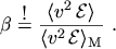
In analogy to statistical mathematics a quantity $ \beta _n$ called kurtosis has been introduced, which is in this work defined as the deviation of the fourth moment of the non-MAXWELL distribution function from the fourth moment of a MAXWELL distribution function with the same standard deviation

$\displaystyle \beta \overset{\textstyle !}{=} \frac{\ensuremath{\langle v^2 \, ...
...l{E} \rangle}} {\ensuremath{\langle v^2 \, \mathcal{E} \rangle}_\mathrm{M}} \ .$ (2.174)

The system is now closed at $ \ensuremath{\langle \phi_6 \rangle}$. Eqn. (2.126) is one possible closure relation obtained from a MAXWELL distribution function. Other empirical closures are also possible (eqn. (2.176)). By introducing an additional temperature $ \Theta_n$2.11

$\displaystyle \Theta_n = T_n \, \beta_n \ ,$ (2.175)

the third power of the temperature $ T_n$ in eqn. (2.126) is substituted by empirically combining different powers of $ T_n$ and $ \Theta_n$

$\displaystyle M_6 = T_n^{3 - i} \, \Theta_n^i \equiv T_n^3 \, \beta_n^i \ , \qquad 0 \leq i \leq 3 \ .$ (2.176)

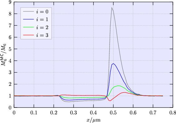
Simulations have shown, that the combination with $ i = 3$ fits best to Monte Carlo data [39, G5]. This is depicted in Fig. 2.4 where the different closure relations are compared with the sixth moment obtained from a Monte Carlo simulation of a one-dimensional $ n^+$-$ n$-$ n^+$ test structure. As can be seen, the closure for the case $ i = 3$ gives the smallest error within the channel. The convergence behavior of the resulting discretized equation system also appeared most stable when using $ i = 3$. Especially for $ i =
1$, which corresponds to closing the system with a MAXWELLian distribution function eqn. (2.126) [40] the NEWTON procedure failed to converge in most cases.

Figure 2.4: Comparison of the different closure relations with the sixth moment from a Monte Carlo simulation.
\includegraphics{gpfigure/Closure.color.eps}

Using $ i = 3$ the closure relation becomes

$\displaystyle \ensuremath{\langle \phi_6 \rangle}= \frac{7 \ensuremath{\cdot}5 ...
...h{\cdot}3}{2} \, \frac{\mathrm{k}_\mathrm{B}^3}{m^2} \, n \, T_n^3 \, \beta_n^3$ (2.177)

and the full six moments transport model reads

$\displaystyle \ensuremath{\ensuremath{\ensuremath{\boldsymbol{\mathrm{\nabla}}}}\ensuremath{\cdot}\ensuremath{\boldsymbol{\mathrm{J}}}_n}$ $\displaystyle = \mathrm{q}\, (R + \ensuremath{\partial_{t} \, n}) \ ,$ (2.178)
$\displaystyle \ensuremath{\boldsymbol{\mathrm{J}}}_n$ $\displaystyle = \mu_n \, \mathrm{k}_\mathrm{B}\, \Bigl( \ensuremath{\ensuremath...
...}{\mathrm{k}_\mathrm{B}} \, \ensuremath{\boldsymbol{\mathrm{E}}}\, n \Bigr) \ ,$ (2.179)

$\displaystyle \ensuremath{\ensuremath{\ensuremath{\boldsymbol{\mathrm{\nabla}}}}\ensuremath{\cdot}\ensuremath{\boldsymbol{\mathrm{S}}}_n}$ $\displaystyle = - \frac{3}{2} \, \mathrm{k}_\mathrm{B}\, \ensuremath{\partial_{...
...B}\, n \, \frac{T_n - T_\mathrm{L}}{\tau_\mathcal{E}} + G_{\mathcal{E}\, n} \ ,$ (2.180)
$\displaystyle \ensuremath{\boldsymbol{\mathrm{S}}}_n$ $\displaystyle = - \frac{5}{2} \, \frac{\mathrm{k}_\mathrm{B}^2}{\mathrm{q}} \, ...
...rm{k}_\mathrm{B}} \, \ensuremath{\boldsymbol{\mathrm{E}}}\, n \, T_n \Bigr) \ ,$ (2.181)

$\displaystyle \ensuremath{\ensuremath{\ensuremath{\boldsymbol{\mathrm{\nabla}}}}\ensuremath{\cdot}\ensuremath{\boldsymbol{\mathrm{K}}}_n}$ $\displaystyle = - \frac{15}{4} \, \mathrm{k}_\mathrm{B}^2 \, \ensuremath{\parti...
... n \, \frac{T_n^2 \, \beta_n - T_\mathrm{L}^2}{\tau_\beta} + G_{\beta \, n} \ ,$ (2.182)
$\displaystyle \ensuremath{\boldsymbol{\mathrm{K}}}_n$ $\displaystyle = - \frac{35}{4} \, \frac{\mathrm{k}_\mathrm{B}^3}{\mathrm{q}} \,...
...{B}} \, \ensuremath{\boldsymbol{\mathrm{E}}}\, n \, T_n^2 \, \beta_n \Bigr) \ .$ (2.183)

In the following the equations for the six moments transport model are rewritten by introducing the charge sign $ s_n$ for electrons and the coefficients $ C_1$ to $ C_5$. The balance equations become

$\displaystyle \ensuremath{\ensuremath{\ensuremath{\boldsymbol{\mathrm{\nabla}}}}\ensuremath{\cdot}\ensuremath{\boldsymbol{\mathrm{J}}}_n}$ $\displaystyle = - s_n \, \mathrm{q}\, (\ensuremath{\partial_{t} \, n}$           $\displaystyle + R) \ ,$ (2.184)
$\displaystyle \ensuremath{\ensuremath{\ensuremath{\boldsymbol{\mathrm{\nabla}}}}\ensuremath{\cdot}\ensuremath{\boldsymbol{\mathrm{S}}}_n}$ $\displaystyle = - \mathrm{C}_2 \, \ensuremath{\partial_{t} \, (n \, T_n)}$   $\displaystyle + \ensuremath{\boldsymbol{\mathrm{E}}}\ensuremath{\cdot}\ensuremath{\boldsymbol{\mathrm{J}}}_n$   $\displaystyle - \mathrm{C}_2 \, n \, \frac{T_n - T_\mathrm{L}}{\tau_\mathcal{E}}$   $\displaystyle + G_{\mathcal{E}\, n} \ ,$ (2.185)
$\displaystyle \ensuremath{\ensuremath{\ensuremath{\boldsymbol{\mathrm{\nabla}}}}\ensuremath{\cdot}\ensuremath{\boldsymbol{\mathrm{K}}}_n}$ $\displaystyle = - \mathrm{C}_4 \, \ensuremath{\partial_{t} \, (n \, T_n^2 \, \beta_n)}$   $\displaystyle + 2 \, s_n \, \mathrm{q}\, \ensuremath{\boldsymbol{\mathrm{E}}}\ensuremath{\cdot}\ensuremath{\boldsymbol{\mathrm{S}}}_n$   $\displaystyle - \mathrm{C}_4 \, n \, \frac{T_n^2 \, \beta_n - T_\mathrm{L}^2}{\tau_\beta}$   $\displaystyle + G_{\beta \, n} \ ,$ (2.186)

with

$\displaystyle \mathrm{C}_2 = \frac{3}{2} \, \mathrm{k}_\mathrm{B}\ , \textcolor{lightgrey}{.......}\mathrm{C}_4 = \frac{15}{4} \, \mathrm{k}_\mathrm{B}^2$ (2.187)

and the following flux equations:

$\displaystyle \ensuremath{\boldsymbol{\mathrm{J}}}_n$ $\displaystyle = - \mathrm{C}_1 \, \Bigl( \ensuremath{\ensuremath{\ensuremath{\boldsymbol{\mathrm{\nabla}}}}\, (n \, T_n)}$   $\displaystyle - s_n \, \frac{\mathrm{q}}{\mathrm{k}_\mathrm{B}} \, \ensuremath{\boldsymbol{\mathrm{E}}}\, n \Bigr) \ ,$ $\displaystyle \textcolor{lightgrey}{.......}\mathrm{C}_1$ $\displaystyle = s_n \, \mathrm{k}_\mathrm{B}\, \mu_n \ ,$ (2.188)
$\displaystyle \ensuremath{\boldsymbol{\mathrm{S}}}_n$ $\displaystyle = - \mathrm{C}_3 \, \Bigl( \ensuremath{\ensuremath{\ensuremath{\boldsymbol{\mathrm{\nabla}}}}\, (n \, T_n^2 \, \beta_n)}$   $\displaystyle - s_n \, \frac{\mathrm{q}}{\mathrm{k}_\mathrm{B}} \, \ensuremath{\boldsymbol{\mathrm{E}}}\, n \, T_n \Bigr) \ ,$ $\displaystyle \textcolor{lightgrey}{.......}\mathrm{C}_3$ $\displaystyle = \frac{5}{2} \, \frac{\mathrm{k}_\mathrm{B}^2}{\mathrm{q}} \, \frac{\tau_S}{\tau_m} \, \mu_n \ ,$ (2.189)
$\displaystyle \ensuremath{\boldsymbol{\mathrm{K}}}_n$ $\displaystyle = - \mathrm{C}_5 \, \Bigl( \ensuremath{\ensuremath{\ensuremath{\boldsymbol{\mathrm{\nabla}}}}\, (n \, T_n^3 \, \beta_n^3)}$   $\displaystyle - s_n \, \frac{\mathrm{q}}{\mathrm{k}_\mathrm{B}} \, \ensuremath{\boldsymbol{\mathrm{E}}}\, n \, T_n^2 \, \beta_n \Bigr) \ ,$ $\displaystyle \textcolor{lightgrey}{.......}\mathrm{C}_5$ $\displaystyle = \frac{35}{4} \, \frac{\mathrm{k}_\mathrm{B}^3}{\mathrm{q}} \, \frac{\tau_K}{\tau_m} \, \mu_n \ .$ (2.190)

The equations for holes are obtained by replacing $ n$ by $ p$ and taking into account that $ s_p
= 1$:

$\displaystyle \ensuremath{\ensuremath{\ensuremath{\boldsymbol{\mathrm{\nabla}}}}\ensuremath{\cdot}\ensuremath{\boldsymbol{\mathrm{J}}}_p}$ $\displaystyle = - \mathrm{q}\, (R + \ensuremath{\partial_{t} \, p}) \ ,$ (2.191)
$\displaystyle \ensuremath{\boldsymbol{\mathrm{J}}}_p$ $\displaystyle = - \mu_p \, \mathrm{k}_\mathrm{B}\, \Bigl( \ensuremath{\ensurema...
...}{\mathrm{k}_\mathrm{B}} \, \ensuremath{\boldsymbol{\mathrm{E}}}\, p \Bigr) \ ,$ (2.192)

$\displaystyle \ensuremath{\ensuremath{\ensuremath{\boldsymbol{\mathrm{\nabla}}}}\ensuremath{\cdot}\ensuremath{\boldsymbol{\mathrm{S}}}_p}$ $\displaystyle = - \frac{3}{2} \, \mathrm{k}_\mathrm{B}\, \ensuremath{\partial_{...
...B}\, p \, \frac{T_p - T_\mathrm{L}}{\tau_\mathcal{E}} + G_{\mathcal{E}\, p} \ ,$ (2.193)
$\displaystyle \ensuremath{\boldsymbol{\mathrm{S}}}_p$ $\displaystyle = - \frac{5}{2} \, \frac{\mathrm{k}_\mathrm{B}^2}{\mathrm{q}} \, ...
...rm{k}_\mathrm{B}} \, \ensuremath{\boldsymbol{\mathrm{E}}}\, p \, T_p \Bigr) \ ,$ (2.194)

$\displaystyle \ensuremath{\ensuremath{\ensuremath{\boldsymbol{\mathrm{\nabla}}}}\ensuremath{\cdot}\ensuremath{\boldsymbol{\mathrm{K}}}_p}$ $\displaystyle = - \frac{15}{4} \, \mathrm{k}_\mathrm{B}^2 \, \ensuremath{\parti...
... p \, \frac{T_p^2 \, \beta_p - T_\mathrm{L}^2}{\tau_\beta} + G_{\beta \, p} \ ,$ (2.195)
$\displaystyle \ensuremath{\boldsymbol{\mathrm{K}}}_p$ $\displaystyle = - \frac{35}{4} \, \frac{\mathrm{k}_\mathrm{B}^3}{\mathrm{q}} \,...
...{B}} \, \ensuremath{\boldsymbol{\mathrm{E}}}\, p \, T_p^2 \, \beta_p \Bigr) \ .$ (2.196)

M. Gritsch: Numerical Modeling of Silicon-on-Insulator MOSFETs PDF