The numerical evaluation of a volume integral over an arbitrary tetrahedron
should, if possible, be widely avoided. Under different circumstances this rule
of thumb cannot be fulfilled and the software engineer rely on a computational
evaluation. In this case it is highly recommended to use existing code or
libraries as described in Section B.3.4. Nevertheless, the
following gives a rough sketch of a possible numerical volume
integral evaluation.
 |
(B.11) |
 |
(B.12) | ||
 |
(B.13) |
| (B.14) |
 |
(B.15) |
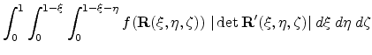
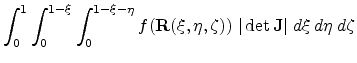
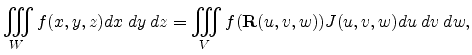
The volume integral over an arbitrary tetrahedron mapped to a standard
![]() -simplex can now be written as
-simplex can now be written as
Numerical integration methods can generally be described as combining
evaluations of the integrand to get an approximation of the integral. An
important part of the analysis of any numerical integration method is to study
the behavior of the approximation error as a function of the number of
integrand evaluations. A method which yields a small error for a small number
of evaluations is usually considered superior. Reducing the number of
evaluations of the integrand reduces the number of arithmetic operations
involved, and therefore reduces the total round-off error. Also, each
evaluation consumes time and the integrand may be arbitrarily complicated.
A large class of quadrature rules can be derived by constructing interpolating
functions which are easy to integrate. Typically these interpolating functions
are polynomials. The Newton-Cotes formulas (named after Isaac
Newton and Roger Cotes) are
a group of formulas for numerical integration. It is assumed that
the value of a function ![]() is known at equally spaced points
is known at equally spaced points ![]() , for
, for
![]() . If the evaluation points are not assumed to be equally spaced,
another class of formulas, called Gausssian quadrature, can be derived.
With the Gaussian quadrature rule an exact result for polynomials of degree
. If the evaluation points are not assumed to be equally spaced,
another class of formulas, called Gausssian quadrature, can be derived.
With the Gaussian quadrature rule an exact result for polynomials of degree
![]() , by a suitable choice of the
, by a suitable choice of the ![]() points
points ![]() and weights
and weights ![]() can be
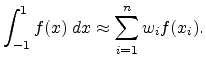
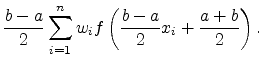
achieved. The domain of integration for such a rule is conventionally taken as
can be
achieved. The domain of integration for such a rule is conventionally taken as
![]() , so the rule is stated as
, so the rule is stated as
Table B.1 gives an
overview of some polynomials used for the more general Gaussian quadrature
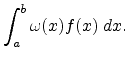
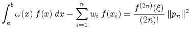
where by introducing a weight function
![]() into the integrand and allowing
interval others than
into the integrand and allowing
interval others than ![]() the problem is given by
the problem is given by
 |
(B.19) |
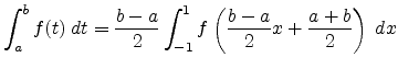
If an integral within the interval ![]() must be changed into an integral
with the limits
must be changed into an integral
with the limits ![]() , the following transformation can be
applied:
, the following transformation can be
applied:
 |
(B.20) |
 |
(B.21) |
The error of a Gaussian quadrature rule can be stated as follows. For an
integrand with ![]() continuous derivatives,
continuous derivatives,
 |
(B.22) |
For a quadrature approximation of the volume integral given in
formula (B.15), one has to take into account that the points of
evaluation reflect the nature of the integration volume. For
example, for an integration along the ![]() coordinate, the
according differential volume slice of the standard
coordinate, the
according differential volume slice of the standard ![]() -simplex gets smaller and
smaller with increasing
-simplex gets smaller and
smaller with increasing ![]() values. A common way of integration
is to reduce the problem from a simplex to an integration over a
cube [138,139]. A general extension of this approach regarding
the standard
values. A common way of integration
is to reduce the problem from a simplex to an integration over a
cube [138,139]. A general extension of this approach regarding
the standard ![]() -simplex is given in [140]. Based on the work given
in [141] the polynomial class of Legendre polynomials is chosen for
the quadrature of a standard
-simplex is given in [140]. Based on the work given
in [141] the polynomial class of Legendre polynomials is chosen for
the quadrature of a standard ![]() -simplex mapped on a cube.
-simplex mapped on a cube.
An integral over the standard ![]() -simplex may be written as
-simplex may be written as
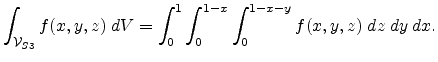 |
(B.23) |
| (B.25) |
and finally a Gaussian quadrature based on Legendre polynomials can now be used to solve
formula (B.24).
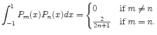
Legendre polynomials are solutions of Legendre's differential equation defined as
![$\displaystyle \frac{d}{dx} \left[ (1-x^2) \frac{d}{dx} P(x) \right] + n(n+1)P(x) = 0.$](img671.png) |
(B.27) |
Each Legendre polynomial ![]() has degree
has degree ![]() and is
expressed via
and is
expressed via
![$\displaystyle P_n(x) = (2^n n!)^{-1} \frac{d^n}{dx^n } \left[ (x^2 -1)^n \right].$](img676.png) |
(B.28) |
 |
(B.29) |
The first few Legendre polynomials are
and their roots
![]() can be found numerically by well-known
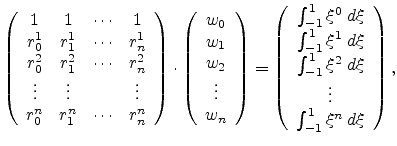
methods [142]. According to formula (B.16), for
the weights
can be found numerically by well-known
methods [142]. According to formula (B.16), for
the weights
![]() one has to solve the linear system given as
follows:
one has to solve the linear system given as
follows:
Due to the wide spectrum of numerical integration problems, approaches are
multifaceted. Several libraries (under different licenses) are available
offering more or less out of the box solutions for the problems depicted in this
chapter. To give a short indication for further investigations, two libraries
are presented.
For a direct evaluation of integrals over the standard ![]() -simplex the
Numerical Algorithm Group (NAG) [143] library routine D01PAF can
be used. This routine returns a sequence of approximations to the integral of a
function over a
multi-dimensional simplex, together with an error estimate for the last
approximation. This method is primary based on the work given
in [144,145]. The computational costs depend mostly on the number of
function evaluations, which in turn depends mostly on
the highest computed order of the integral approximation
-simplex the
Numerical Algorithm Group (NAG) [143] library routine D01PAF can
be used. This routine returns a sequence of approximations to the integral of a
function over a
multi-dimensional simplex, together with an error estimate for the last
approximation. This method is primary based on the work given
in [144,145]. The computational costs depend mostly on the number of
function evaluations, which in turn depends mostly on
the highest computed order of the integral approximation ![]() and
the number of dimensions
and
the number of dimensions ![]() for the integral. The number of function calls
can be estimated by
for the integral. The number of function calls
can be estimated by
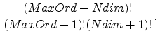 |
(B.32) |
Another very popular library which offers several different numerical quadrature algorithms, mostly based on polynomial integration schemes, is the so-called GNU Scientific Library (GSL) [146]. This library is a collection of routines for numerical computing. The routines have been written in C and present a modern Applications Programming Interface (API) for C programmers, allowing wrappers to be written for high level languages. The source code is distributed under the GNU General Public License.