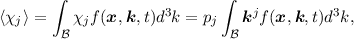
In order to fully analyze semiconductor devices such as metal-oxide-semiconductor field-effect transistors (MOSFET), one needs to solve a coupled system of equations consisting of the Poisson equation and the BTE for electrons and holes. A direct discretization yields a system of equations in seven dimensions. Thus simpler models, which at least capture the essential features of the BTE are often used. One of these methods by which plenty of charge transport models can be obtained is the method of moments [32, 33]. The jth moment of the BTE is defined as
|
| (2.37) |
where χj is the jth weight function and pj is the prefactor of the jth weight function. Table 2.2 lists a few important moments of the distribution function. It is important to note that the moments of the distribution function infer no assumptions and are used to obtain macroscopic quantities often employed in the analysis of the performance of semiconductor devices.
| Moment | χj | Formula | Macroscopic Quantity |
| ⟨χ0⟩ | χ0 = 1 | 1∫
 f(x,k,t)d3k f(x,k,t)d3k | n or p |
| ⟨χ1⟩ | χ1 = k | ℏ ∫
f(x,k,t)kd3k | ⟨v⟩ = Jn∕p∕q |
| ⟨χ2⟩ | χ2 = E(k) | ∫
E(k)f(x,k,t)k2d3k | ⟨En∕p⟩ |
| … | … | … | |
| Table 2.2: | A list of the first few moments of the distribution function, where n and p are the electron and hole concentrations, Jn∕p is the current density and ⟨En∕p⟩ is the average carrier energy for electrons and holes respectively. |
To obtain equations for the moments of the BTE, such as the drift diffusion (DD) model, the BTE is multiplied by increasing orders of the wave vector k and a scalar prefactor p and afterwards integrated over the Brillouin zone
 | (2.38) |
In order to analytically evaluate the integrals over the free-streaming operator and the scattering operator further assumptions are necessary. Since the integral over the free streaming operator in Equation (2.38) would lead to a tensor equation for odd weight functions, identified by an odd index j, a further assumption is needed. This assumption has to be chosen such that all tensors after integration on the left-hand side of Equation (2.38) are diagonal with equal entries along the diagonal. It turns out that it is sufficient to decompose the distribution function into a symmetric and antisymmetric part,
| f(x,k,t) | = fS(x,k,t) + fA(x,k,t), | ||
| fS(x,k,t) | = fS(x,-k,t), | ||
| fA(x,-k,t) | = -fA(x,k,t), |
 |
as well as
 |
which yields a single unique equation per moment [34]. These assumptions are termed diffusion approximation, since it assumes that diffusion of carriers dominates over carrier drift, caused by an electric field. To analytically evaluate the right hand side of Equation (2.38), the relaxation time approximation (RTA) is often utilized. The main assumption of the RTA is that due to scattering the distribution function will relax exponentially into the equilibrium distribution function feq(x,k,t),
 |
where the transition is characterized by a scattering process dependent relaxation time constant τs [22]. This approximation also implies, as can be shown [22], that the relaxation time constants of various scattering processes can be added up to a single time constant as follows:
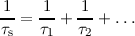 |
After employing all of the assumptions, detailed above, one will obtain an infinite enumerable number of equations. The equation for the jth moment will always contain the j + 1 moment. Thus the array of equations needs to be terminated by replacing the equation for the j + 1 moment with an analytic formula. Such an analytic formula is termed closure condition, which is also the major drawback of any transport model obtained through the method of moments.
The drift diffusion (DD) model is one of the simplest and earliest numerically used and investigated charge transport models [35]. It is obtained by employing the parabolic band approximation (cf. Section 2.1) under the additional assumption of a single conduction and a single valence band. Evaluating the first two moments of the BTE one obtains,
| ⟨χ0⟩ | ⇒ ∂tn -∥q∥-1∇J n - R = 0, | (2.39) |
| ⟨χ0⟩ | ⇒ ∂tp + ∥q∥-1∇J p + R = 0, | (2.40) |
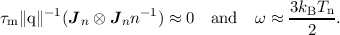
| ⟨χ1⟩ | ⇒ τm∂tJn -∥q∥τmkB∇⋅ + m*J
n = 0, + m*J
n = 0, | (2.41) |
| ⟨χ1⟩ | ⇒ τm∂tJp + ∥q∥τmkB∇⋅ - m*J
p = 0, - m*J
p = 0, | (2.42) |
 | (2.43) |
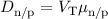
is used as a closure condition, τm is the momentum relaxation time constant, Tn and Tp are the electron and hole temperatures respectively and R is a scalar term accounting for electron/hole recombination and generation. In order to further simplify the DD model, the influence of the time derivative of the current density is often neglected, which is justified if the frequency of the electric field E is two times lower than the plasma frequency [36]. Thus, including Poisson’s equation to calculate the electric field, the DD model reads
∇⋅ | = ∥q∥(n - p + C), | (2.44) |
| ∥q∥∂tn -∇Jn | = ∥q∥R, | (2.45) |
| ∥q∥∂tp + ∇Jp | = -∥q∥R, | (2.46) |
Jn =  μnkB μnkB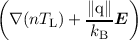 | =  drift term + drift term +  diffusion term, diffusion term, | (2.47) |
Jp =  μpkB μpkB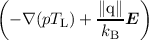 | = ∥q∥μpE -∥q∥Dp∇p, | (2.48) |
 |
have been used. Upon employing this method, one looses exact information regarding the kinetic energy and momentum (k) of the charge carriers and their distribution. Although various material, field and doping dependent models for carrier mobilities have been developed [35], the DD model still suffers from many of the assumptions needed in the course of its derivation. As such, a consequence of setting the lattice temperature and carrier temperature equal is that carrier diffusion will be underestimated by the model. Additionally, by employing the equipartition theorem or its enhancement, the homogeneous energy balance equation [34], to calculate the average carrier energy it is not possible to describe effects of rapidly changing electric fields. Thus it is for example not possible to explain the phenomenon of velocity overshoot [37] and energy transport phenomena using the DD model. Nevertheless, because of its ease to comprehend and compact formulation, the DD model is the best known and most widely used charge transport model today.
The hydrodynamic model (HD), first developed by [32, 33], is derived like the DD model by employing the method of moments. Instead of using only the first two moments of the BTE, the HD model uses the first three moments in order to incorporate spatial dependencies on the average carrier energy, thereby adding two new unknowns and at least one new parameter. As a closure condition Fourier’s law is used for the fourth moment. In addition the initial assumption that
 |
is dropped in the HD model, which reads
κ is given by the Wiedemann-Franz law, τE is the energy relaxation time, nSn is the carrier heat flux (third moment), ω is the average carrier energy and ω0 is the equilibrium average carrier energy. For holes a similar set of equations is obtained. A simplified version of the HD model, the energy transport model, can be obtained by assuming that
 | (2.54) |
The benefit of the HD model over the DD model is, that it can describe velocity overshoot, although it can only cover processes which can be explained by employing heated Maxwellian distribution functions. Upon investigating this property of the HD model it was found that one can observe an artificial velocity overshoot for decreasing electric fields too [38]. Sadly, it was also found that this is due to the truncation after the 4th moment in the construction of the model and thus an intrinsic property of the HD model [38]. Additionally, the HD model tends to overestimate the number of carriers in the bulk of MOSFETs. In addition to all that the equations of the HD model are strongly hyperbolic, which makes them numerically challenging to solve for arbitrary device geometries.
Higher order charge transport models have been developed in hope to overcome the limitations of the hydrodynamic model. The most notable one is the Six Moments model, where the closure condition is obtained through an empirical relation [39]. Although higher order models capture more of the essential physics described by the BTE they also tend to be more complex, have more parameters and are harder to understand, derive and implement. The increased complexity in these models often, despite successfully describing many transport effects observed in semiconductors, trades off the benefit of the more accurate description.
