
The Monte Carlo method itself is a stochastic algorithm to solve integral equations [40, 25, 41]. Since the BTE can be formally transformed into an integral equation, the Monte Carlo (MC) method provides a way to solve the BTE. The main idea of the MC method for the BTE is to simulate the flow (cf. Figure 2.4) of a statistically representative ensemble of particles by following the path of each single particle. In between scattering events each particle propagates freely according to
|
| (2.55) |
while scattering events are determined stochastically and occur instantly. In order to determine the instance of a scattering event one starts from the formally integrated BTE. From this form one can, through algebraic transformations, obtain the conditional probability density p(x,k,ν,t0 + T|x0,k0,ν0,t0) to find a particle (electron or hole), without being scattered, in state (x,k,ν) at time t0 + T after it has been at time t0 in state (x0,k0,ν0). Now p(x0,k0,ν0,t0|x,k,ν,t0 + T) is evaluated using random numbers to determine whether or not a particle is scattered, giving the method its name and characteristics (cf. Figure 2.7).
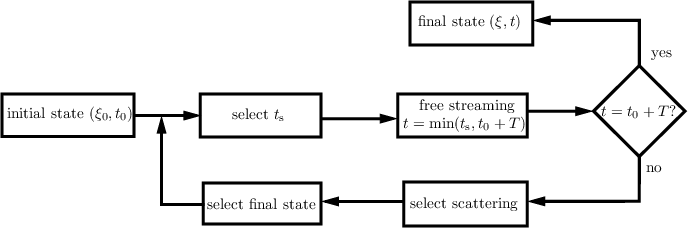
| Figure 2.7: | A flowchart of the Monte Carlo method for solving the BTE in time T, where ξ = (x,k,ν) and ts is the time at which the next scattering event occurs. Reproduced from [25]. |
It is important to state that by using the MC method it is possible to directly solve the uncoupled (no recombination or generation) BTEs for electrons and holes self-consistently with Poisson’s equation (cf. Equation (2.27)). By virtue of the method it is not necessary to approximate the bandstructure Eν(k) of the semiconductor and it is indeed straightforward to incorporate the full dispersion relation into a simulator using the MC method. Additionally, one can directly obtain fνn and fνp from any MC simulator by averaging over all particles and thus calculate the moments by evaluating the respective integrals numerically (cf. Section 2.3). This is indeed very satisfying, since a maximum of physically relevant and accurate information can in principle be obtained by a minimum of approximations. Nevertheless, approximations to the BTE are necessary. In order to be able to apply the MC method, the BTE needs to be linearized [25]. This linearization in turn requires one to drop Pauli’s exclusion principle in the scattering operator and also severely impacts the ability to rigorously implement non-linear scattering operators such as electron-electron scattering. However, electron-electron scattering in Monte Carlo based device simulators, using a plethora of approximations, has been implemented for 1D device geometries [42, 43]. Additionally, in order for the MC method to yield useful results very large numbers of particles are required in a simulation, since the accuracy in fν(x,k,t) exhibits a square root dependence on the number of particles [44]. Large ensembles of particles in turn lead to a large computational burden, such that significant MC simulations can take from a few hours up to several workdays or even months to complete. The reason for this unfortunate property is due to the stochastic nature of any MC method, which can even be easily observed in simple simulations. In Figure 2.9, the electron distribution function fn for a n+-n-n+ structure (cf. Figure 2.8) obtained by using the MC simulator MONJU [45] is presented. The numeric noise towards higher kinetic energies is clearly visible.
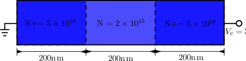
| Figure 2.8: | The exemplary 2D n+-n-n+ structure simulated using MONJU [45]. The structure is 100nm wide. |
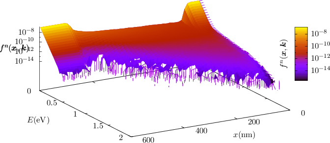
| Figure 2.9: | The electron distribution function plotted over the long side of the n+-n-n+ diode, obtained by full-band MC simulation using MONJU [45]. The numeric noise towards higher kinetic energies is clearly visible. In the simulation, which took one workday to complete, five million particles have been used. |