![\includegraphics[width=2.2in,angle=0]{figures/Si_lattice.eps}](img222.png)
![\includegraphics[width=3.2in,angle=0]{figures/BZ4.eps}](img223.png)
![]()
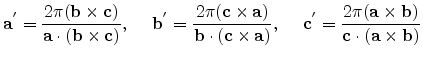
The Bravais lattice vectors for Si are given by
| (3.32) |
 |
(3.33) |
![$\displaystyle {\mathbf{a}}' = \frac{2\pi}{a_0}[\overline{1},1,1]^{T}, \hspace*{...
...},1]^{T}, \hspace*{5mm} {\mathbf{c}}' = \frac{2\pi}{a_0}[1,1,\overline{1}]^{T}.$](img234.png) |
(3.34) |
The first Brillouin zone has the shape of a truncated octahedron. It can be
visualized as a set of eight hexagonal planes halfway between the centre of the
cell and the lattice points at the corner, and six square planes halfway to the
lattice points in the center of the next cell. The Brillouin zone is shown in
Fig. 3.4b with the points and directions of high-symmetry marked
using Greek letters and Roman letters for points on the
surface. Table 3.3 summarizes these symmetry points and
directions. These points and directions are of importance for interpreting the
band structure plots.
| Symmetric Points/ | ||
| Directions | Coordinate | Remark |
| ( |
Origin of k space | |
| ( |
Middle of square faces | |
|
|
Middle of hexagonal faces | |
|
|
Middle of edge shared by two hexagons | |
| Middle of edge shared by a hexagons and a square | ||
| Middle of edge shared by two hexagons and a square | ||
|
|
Directed from |
|
|
|
Directed from |
|
|
|
|
Directed from |
Several symmetry operations can be performed on the diamond structure which leave the structure unchanged. Apart from translation, such operations can be categorized as rotation or inversion, or a combination, and are collectively known as symmetry operations. Due to the fcc lattice of the diamond structure there exist a total of 48 such independent symmetry operations. This symmetry of the lattice in real space is also reflected in the first BZ. The lowering of symmetry of the fcc structure due to strain can distort it to some of the 14 Bravais lattice forms, such as the tetragonal, orthorhombic or trigonal lattice. The new lattice structure formed has different symmetry properties which can have pronounced consequences on the band structure. Numerical methods for calculating the band structure allow the prediction of several important electronic and optical properties.
![\includegraphics[width=3.0in,angle=0]{figures/enzo_Si_bandstructure_new.eps}](img251.png)
![\includegraphics[width=3.0in,angle=0]{figures/enzo_Si_Vbandstructure_new.eps}](img252.png)
![]()
The numerical band structure of unstrained Si calculated using the empirical pseudopotential method
[Chelikowsky76] is shown in Fig. 3.5. At ![]() , the
highest energy band that is completely filled is denoted as the valence
band. The next higher band is completely empty at
, the
highest energy band that is completely filled is denoted as the valence
band. The next higher band is completely empty at ![]() and called the
conduction band. The two bands are separated by a forbidden energy gap, known
as the bandgap
and called the
conduction band. The two bands are separated by a forbidden energy gap, known
as the bandgap ![]() .
.
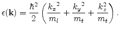
The principal conduction band minima of Si are located along the ![]() ,
,
![]() and
and ![]() directions at a distance of about 85% from the
directions at a distance of about 85% from the
![]() -point to the X-points. The minima of the second conduction band touch
the first conduction band at the X-points. This degeneracy of the two
conduction bands can produce interesting effects on applying shear strain as
discussed in Section 3.3.4. Close to the principal
minima the band structure can be represented by ellipsoidal constant energy
surfaces by assuming a parabolic energy dispersion relation, as shown
in Fig. 3.6a. For valleys located along the [100] direction, the
energy dispersion reads
-point to the X-points. The minima of the second conduction band touch
the first conduction band at the X-points. This degeneracy of the two
conduction bands can produce interesting effects on applying shear strain as
discussed in Section 3.3.4. Close to the principal
minima the band structure can be represented by ellipsoidal constant energy
surfaces by assuming a parabolic energy dispersion relation, as shown
in Fig. 3.6a. For valleys located along the [100] direction, the
energy dispersion reads
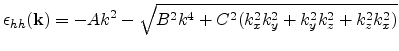
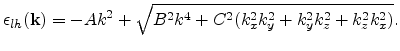
Unlike the conduction band, the valence band structure looks highly anisotropic
even in the unstrained case. The valence band maximum in Si is located at
the ![]() point. Due to the degeneracy of the bands at the
point. Due to the degeneracy of the bands at the ![]() point,
the energy surfaces develop into quartic surfaces of the
form [Dresselhaus55]
point,
the energy surfaces develop into quartic surfaces of the
form [Dresselhaus55]
 |
(3.36) |
 |
(3.37) |
![\includegraphics[width=2.4in,angle=0]{figures/Si_Xvalleys_Uns2.eps}](img269.png)
![\includegraphics[width=3.6in,angle=0]{figures/Unstrained3D_HH4.eps}](img270.png)
![]()
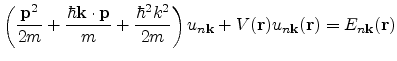
In the
![]() method, the single-electron Schroedinger equation is expanded using
Bloch's theorem, to yield a
method, the single-electron Schroedinger equation is expanded using
Bloch's theorem, to yield a
![]() term and an additional term parabolic in
term and an additional term parabolic in ![]() to
the original equation.
to
the original equation.
 is the momentum operator. The function
A very powerful tool for obtaining the complete band structure is the empirical pseudopotential method. In
this method, the actual hard core ionic potential, ![]() , experienced by an
electron is replaced by a soft pseudopotential,
, experienced by an
electron is replaced by a soft pseudopotential, ![]() . This also results in a
modification of the true wave function,
. This also results in a
modification of the true wave function, ![]() , to a pseudo-function,
, to a pseudo-function, ![]() ,
as shown in Fig. 3.7. The pseudopotential is found to depend on
pseudopotential form factors which can be obtained by matching experimental
results and are available for a large set of material
systems [Yu03]. Knowing this potential, the Schroedinger equation
gets modified to a so called pseudo wave equation, the solution of which
delivers the energy dispersion relation.
,
as shown in Fig. 3.7. The pseudopotential is found to depend on
pseudopotential form factors which can be obtained by matching experimental
results and are available for a large set of material
systems [Yu03]. Knowing this potential, the Schroedinger equation
gets modified to a so called pseudo wave equation, the solution of which
delivers the energy dispersion relation.