Next: 4. Mobility Modeling
Up: 3. Strain Effects on
Previous: 3.2 Structure of Relaxed
Subsections
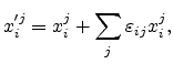
3.3 Effect of Strain
A comprehensive study of the effect of strain on the band structure has been
performed Bir and Pikus [Bir74]. A direct result of straining the crystal
is the transformation of the unstrained lattice vectors ( ) to the
strained lattice vectors (
) to the
strained lattice vectors (
 ), through the relation
 |
(3.39) |
where
 denote the strain tensor components. The effect of
strain can be incorporated into
denote the strain tensor components. The effect of
strain can be incorporated into
 band structure calculations by introducing
an additional perturbation term into the unstrained
potential [Manku93b]. For the empirical pseudopotential method, an interpolation of the
pseudopotential form factors is required. Moreover, in the presence of an
arbitrary strain condition, there occurs a movement of the vertex atoms as well
as the central atom, which results in an ambiguity in the exact location of the
central atom in the bulk strained primitive unit cell. This effect can be
captured by taking into account an additional internal displacement
parameter [de Walle86].
band structure calculations by introducing
an additional perturbation term into the unstrained
potential [Manku93b]. For the empirical pseudopotential method, an interpolation of the
pseudopotential form factors is required. Moreover, in the presence of an
arbitrary strain condition, there occurs a movement of the vertex atoms as well
as the central atom, which results in an ambiguity in the exact location of the
central atom in the bulk strained primitive unit cell. This effect can be
captured by taking into account an additional internal displacement
parameter [de Walle86].
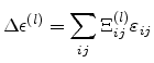
Figure 3.7:
The concept of pseudopotential where the true potential  and
the true wave function
and
the true wave function  are replaced by a pseudopotential
  and a
pseudo wave function
and a
pseudo wave function  .
.
The effect of strain on the conductivity of Si was first investigated by
Smith [Smith54]. The principal finding of his experimental work was the
observation of a change in the Si resistivity on applying uniaxial tensile
stress. This change occurs due to a modification of the electronic band
structure. Microscopically, the modification stems from a reduction in the
number of symmetry operations allowed, which in turn depends on the way the
crystal is stressed. This breaking of the symmetry of the fcc lattice of
Si can result in a shift in the energy levels of the different conduction
and valence bands, their distortion, removal of degeneracy, or any
combination. In the following sections these effects are discussed in detail.
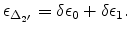
Strain induces a shift in the energy levels of the unstrained conduction and
valence bands. While hydrostatic strain merely shifts the energy levels of a
band, uniaxial and biaxial strain removes the band degeneracy. These energy
shifts can either be extracted from the full-band structure calculated
numerically including strain, or obtained analytically using the linear
deformation potential theory.
3.3.1.1 Deformation Potential Theory
Deformation potential theory originally developed by Bardeen and
Shockley [Bardeen50] was used to investigate the interaction of electrons
with acoustic phonons. It was later generalized to include different scattering
modes by Herring and Vogt [Herring56]. The technique was applied to
strained material systems by Bir and Pikus [Bir74].
Within the framework of this theory, the energy shift of a band extremum  is
expanded in terms of the components of the strain tensor
.
is
expanded in terms of the components of the strain tensor
.
 |
(3.40) |
The tensor quantity  is called the deformation potential. The
symmetry of the strain tensor is also reflected in that of the deformation
potential tensor, giving
is called the deformation potential. The
symmetry of the strain tensor is also reflected in that of the deformation
potential tensor, giving
 |
(3.41) |
The maximum number of independent components of this tensor is six which is
reduced to two or three for a cubic lattice. These are usually denoted by
 , the uniaxial deformation potential constant, and
  , the
dilatation deformation potential constant. The deformation potential constants
can be calculated using theoretical techniques such as density functional
theory [de Walle86], the non-local empirical pseudopotential
method [Fischetti96], or ab-initio calculations. However, a final
adjustment of the potentials is obtained only after comparing the calculated
values with those obtained from measurement techniques.
, the
dilatation deformation potential constant. The deformation potential constants
can be calculated using theoretical techniques such as density functional
theory [de Walle86], the non-local empirical pseudopotential
method [Fischetti96], or ab-initio calculations. However, a final
adjustment of the potentials is obtained only after comparing the calculated
values with those obtained from measurement techniques.
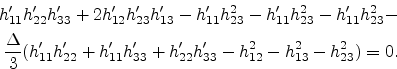
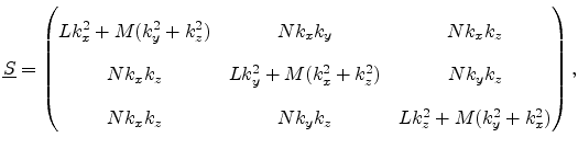
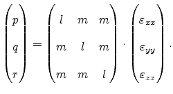
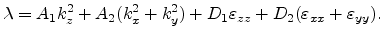
The general form of the strain-induced energy shifts of the conduction band
valleys for an arbitrary strain tensor can be written as
 |
(3.42) |
where
 is a unit vector of the
 valley minimum for the
 (
( ) valley type. The first term,
 in (3.42) shifts the energy level of all the valleys equally and is
proportional to the hydrostatic strain,
in (3.42) shifts the energy level of all the valleys equally and is
proportional to the hydrostatic strain,
 . The difference in the energy levels of
the valleys arises from the second term in (3.42). The analytical
expressions for this term for different stress directions is listed in
Table 3.4.
. The difference in the energy levels of
the valleys arises from the second term in (3.42). The analytical
expressions for this term for different stress directions is listed in
Table 3.4.
Due to the degeneracy of the valence bands, strain induced splitting of the
bands cannot be calculated as straight forwardly as for the conduction
bands. The energy shifts can be calculated from the
theory in conjunction
with the deformation potential theory. The energy dispersion of the valence
bands is obtained from of a perturbation matrix
 and a deformation
potential matrix
and a deformation
potential matrix

 |
(3.43) |
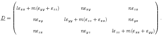 |
(3.44) |
The parameters  are related to the Luttinger
parameters [Yu03] while
are related to the Luttinger
parameters [Yu03] while  denote valence band deformation
potentials. The effect of spin-orbit coupling is taken into account by
introducing a spin-orbit interaction term,
denote valence band deformation
potentials. The effect of spin-orbit coupling is taken into account by
introducing a spin-orbit interaction term,
 , dependent on the
unstrained energy level
, dependent on the
unstrained energy level  , of the split off band, as an additional
perturbation into the Hamiltonian,
, of the split off band, as an additional
perturbation into the Hamiltonian,
 |
(3.45) |
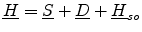
After performing a unitary transformation on
 followed by some
mathematical manipulations, Manku [Manku93b] arrived at the following
form to describe the valence band spectrum.
followed by some
mathematical manipulations, Manku [Manku93b] arrived at the following
form to describe the valence band spectrum.
Here the  and the
  are related to the matrices
and
through the relation
are related to the matrices
and
through the relation
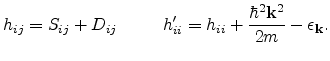 |
(3.47) |
Equation (3.47) can be simplified to
 |
(3.48) |
which is a cubic equation in  . Its solutions give the energies for the HH,
LH and the SO bands for a particular k value and arbitrary strain. The
components
. Its solutions give the energies for the HH,
LH and the SO bands for a particular k value and arbitrary strain. The
components  are functions of the strain tensor. Unlike the work of Bir
and Pikus where the spin orbit coupling was neglected, the expression
in (3.49) has been derived taking into account this interaction as an
additional perturbation. The splitting of the bands can be obtained by setting
are functions of the strain tensor. Unlike the work of Bir
and Pikus where the spin orbit coupling was neglected, the expression
in (3.49) has been derived taking into account this interaction as an
additional perturbation. The splitting of the bands can be obtained by setting
 in (3.49) to give
 |
(3.49) |
where the coefficients  are given as
 |
(3.50) |
 |
(3.51) |
 |
(3.52) |
 |
(3.53) |
 |
(3.54) |
 |
(3.55) |
3.3.3 Different Stress Configurations
In this section stress configurations are discussed in which the stress is
applied along the ![$ [001]$](img256.png) ,
, ![$ [110]$](img208.png) and
and ![$ [111]$](img209.png) directions, as well as an
academic case of stress along the
directions, as well as an
academic case of stress along the ![$ [123]$](img334.png) direction.
direction.
3.3.3.1 Biaxial Stress: Tetragonal Distortion
For the case of biaxial stress in the (001) plane, the 6-fold degenerate
 -valleys in Si are split into a 2-fold degenerate
  valley pair (located along the [001] direction) and a 4-fold degenerate
 valleys pair. In terms of symmetry considerations, this stress
condition is equivalent to applying a uniaxial stress along the [001]
direction. The cubic lattice of Si gets distorted to a tetragonal crystal
system (right parallelopiped with a square base). The number of symmetry
operations for this system is reduced by a factor of 3 compared to the
unstrained case.
valleys pair. In terms of symmetry considerations, this stress
condition is equivalent to applying a uniaxial stress along the [001]
direction. The cubic lattice of Si gets distorted to a tetragonal crystal
system (right parallelopiped with a square base). The number of symmetry
operations for this system is reduced by a factor of 3 compared to the
unstrained case.
Biaxial tensile strain obtained by epitaxially growing Si on relaxed SiGe
results in a lowering of the valleys in energy while the  valleys move up in energy. As a result, the following effects become important:
a) electron transfer from the high energy valleys to the low energy
valleys resulting in increased population of the
valleys. This is indicated by the increased size of the lobes in
Fig. 3.8a. b) Reduced probability of electron scattering from
to , and c) the lowered valleys experience a
smaller effective mass,
valleys move up in energy. As a result, the following effects become important:
a) electron transfer from the high energy valleys to the low energy
valleys resulting in increased population of the
valleys. This is indicated by the increased size of the lobes in
Fig. 3.8a. b) Reduced probability of electron scattering from
to , and c) the lowered valleys experience a
smaller effective mass,  , in the (001) plane.
For the valence bands, the degeneracy of the HH and LH bands at the  point is lifted. The top band moves to a lower hole energy and is HH like,
while the other band moves higher in energy. A schematic of the band splitting
is shown in Fig. 3.8b where the in-plane direction is denoted
as
point is lifted. The top band moves to a lower hole energy and is HH like,
while the other band moves higher in energy. A schematic of the band splitting
is shown in Fig. 3.8b where the in-plane direction is denoted
as ![$ [100]$](img207.png) and the out-of-plane direction as . The curvature of the top
band is higher in the out-of-plane direction as compared to the direction.
and the out-of-plane direction as . The curvature of the top
band is higher in the out-of-plane direction as compared to the direction.
Under the application of a uniaxial stress along the [111] direction, the fcc
lattice of unstrained Si is modified to a trigonal system (rhombohedron with
edges having arbitrary angles). The number of symmetry operations is 12,
reduced by a factor 4 compared to the unstrained case. Because this direction
coincides with the diagonal of the cube, all the  -valleys are
symmetrically oriented with respect to this direction. The resulting strain
tensor thus has equal magnitudes of the diagonal components
(see (3.24)). Shear strain components are also present with
-valleys are
symmetrically oriented with respect to this direction. The resulting strain
tensor thus has equal magnitudes of the diagonal components
(see (3.24)). Shear strain components are also present with
 . Consequently, the degeneracy of the valleys is not lifted
and electrons are populating all the valleys equally. In the valence bands, the
energy dispersion in the [100] and [001] directions are the same. The valence
band splittings can be seen in Fig. 3.9a.
. Consequently, the degeneracy of the valleys is not lifted
and electrons are populating all the valleys equally. In the valence bands, the
energy dispersion in the [100] and [001] directions are the same. The valence
band splittings can be seen in Fig. 3.9a.
![\includegraphics[width=2.3in, angle= -0]{figures/Splitting_Biax.eps}](img341.png)
![\includegraphics[width=2.8in]{figures/m1Galong001_nolabels2_rot.ps}](img342.png)

Figure 3.8:
(a) Conduction and (b) valence band splitting under biaxial tensile
strain in the (001) plane.
![\includegraphics[width=2.8in]{figures/1Galong111_nolabels2_rot.ps}](img344.png)
![\includegraphics[width=2.8in]{figures/1Galong110_nolabels2_rot.ps}](img345.png)

Figure 3.9:
(a) Valence band splitting under uniaxial tensile strain along (a) the
[111] and (b) the [110] direction.
Applying uniaxial stress distorts the lattice to a rectangular
parallelopiped with a rhombic base. The resulting strain tensor has both
diagonal and off-diagonal components, see (3.23). The number of symmetry
operations is reduced to a mere 8. For tensile stress along the [110]
direction, the strain induced valley splittings in the conduction bands are
similar to the biaxial tensile case shown in Fig. 3.8. In the
valence bands, the curvature of the top band in the direction is higher
than in the out-of-plane direction as shown in Fig 3.9b.
Stress along the [123] direction reduces the number of symmetry operations of
the lattice to only 2. The resulting crystal structure is triclinic. The strain
tensor has all components non-zero with the diagonal components being
different. For uniaxial tensile stress, the 3 pairs of valleys in
the conduction band are shifted to different energy levels. Also the curvature
of the top valence band is increased in the [100] direction as compared to the
[001] direction. The conduction and valence band splittings are shown in
Fig. 3.10.
![\includegraphics[width=2.1in, angle= -0]{figures/Splitting_123.eps}](img347.png)
![\includegraphics[width=2.6in]{figures/rot_1Galong123_nolabels2.ps}](img348.png)

Figure 3.10:
(a) Conduction and (b) valence band splitting under biaxial tensile
strain in the [123] direction.
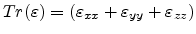
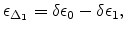
3.3.4 Stress-induced Degeneracy Lifting
The first and second conduction bands are degenerate at the X-point. This
coupling of the two bands at the X-point was understood in terms of the X-ray
scattering results obtained on the diamond
lattice [Bouckaert36]. The effect of strain on the degeneracy of the bands
at the X-point was first examined in the theoretical study performed by Bir and
Pikus [Bir74] and later verified experimentally by Hensel [Hensel65]
and Laude [Laude71].
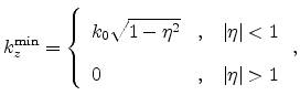
For any stress condition which causes the strain tensor to have non-diagonal
components, there is a distortion of the band structure and the degeneracy at
some of the X-points is lifted. This leads to a change in the electron
effective mass which has been detected using cyclotron resonance
experiments [Hensel65]. We consider the case in which a uniaxial stress is
applied along the [110] direction.
The band splitting at the X-point can be calculated from the solution of the
eigenvalue problem stated in [Hensel65].
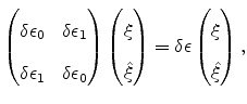 |
(3.56) |
where
The constant  in (3.59) is a new deformation potential
ascribed to the degeneracy lifting at X-point. Two different values of
have been suggested:
in (3.59) is a new deformation potential
ascribed to the degeneracy lifting at X-point. Two different values of
have been suggested: 
 eV predicted from cyclotron
resonance experiments [Hensel65] and
eV predicted from cyclotron
resonance experiments [Hensel65] and  eV from indirect exciton
spectrum measurements [Laude71]. The energy levels of the two conduction
bands are thus given by
eV from indirect exciton
spectrum measurements [Laude71]. The energy levels of the two conduction
bands are thus given by
 |
(3.59) |
 |
(3.60) |
The energy dispersion of the first ( ) and second (
 )
conduction band can be determined from the eigenvalues of the Hamiltonian
suggested by Bir and Pikus [Bir74],
)
conduction band can be determined from the eigenvalues of the Hamiltonian
suggested by Bir and Pikus [Bir74],
 |
(3.61) |
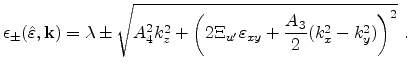
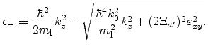
where
 describes the dispersion of and
 that of
, and
that of
, and
 |
(3.62) |
The parameters  to
to  have been obtained in [Ungersboeck07] and are
given as
have been obtained in [Ungersboeck07] and are
given as
where
 |
(3.64) |
and
 denotes the distance of the
conduction band minimum of unstrained Si measured from the
denotes the distance of the
conduction band minimum of unstrained Si measured from the  point. By
adopting a new primed coordinate system that is rotated by 45
point. By
adopting a new primed coordinate system that is rotated by 45 with
respect to the crystallographic coordinate system,
with
respect to the crystallographic coordinate system,
the energy dispersion (3.62) can be written as
 |
(3.66) |
It should be noted that  is invariant under the transformation
described by (3.66). The effective masses in the
is invariant under the transformation
described by (3.66). The effective masses in the ![$ x'=[110]$](img374.png) and
and
![$ y'=[1\bar{1}0]$](img375.png) direction can be obtained using the relations
direction can be obtained using the relations
 |
(3.67) |
 |
(3.68) |
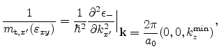
while the longitudinal mass is given by
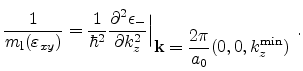 |
(3.69) |
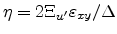
Here
 denotes the minimum of the conduction band
and can be obtained from (3.62). Substituting the values of
to from (3.64) into (3.62) and setting
denotes the minimum of the conduction band
and can be obtained from (3.62). Substituting the values of
to from (3.64) into (3.62) and setting
 , the dispersion relations becomes
 |
(3.70) |
From
 , the position of the
conduction band minimum
is obtained [Ungersboeck07]
, the position of the
conduction band minimum
is obtained [Ungersboeck07]
 |
(3.71) |
where
 . The expression (3.72)
reveals that the minimum in the [001] direction moves closer to the X-point. In
Fig. 3.11, the impact of shear strain on the shape of the
and
conduction bands is plotted. For
. The expression (3.72)
reveals that the minimum in the [001] direction moves closer to the X-point. In
Fig. 3.11, the impact of shear strain on the shape of the
and
conduction bands is plotted. For
 the
position of the minimum is located at the point , thus
the
position of the minimum is located at the point , thus
 , and remains fixed.
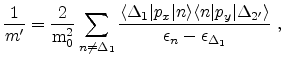
Evaluating the derivatives in (3.68) to (3.70), the strain dependence of
the transversal and longitudinal masses is obtained as
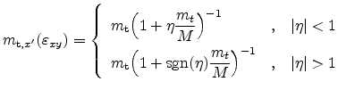 |
(3.72) |
in the direction,
 |
(3.73) |
in
![$ [1\bar{1}0]$](img394.png) direction, and
direction, and
for the longitudinal mass along the direction. Here,
 denotes the signum function and
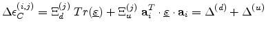
 . This
modification of the band structure translates into a change in the shape of the
constant energy surfaces. The constant energy surfaces of unstrained Si
having a prolate ellipsoidal shape are now deformed to a scalene ellipsoidal
shape, characterized by the masses
. This
modification of the band structure translates into a change in the shape of the
constant energy surfaces. The constant energy surfaces of unstrained Si
having a prolate ellipsoidal shape are now deformed to a scalene ellipsoidal
shape, characterized by the masses  and
and  . As can be seen
from Fig. 3.12, the mass along the stress direction is reduced
whereas perpendicular to the stress direction is increased.
. As can be seen
from Fig. 3.12, the mass along the stress direction is reduced
whereas perpendicular to the stress direction is increased.
![\includegraphics[width=2.5in,angle=0]{figures/mt_circle.eps}](img400.png)
![\includegraphics[width=2.5in,angle=0]{figures/mt_ellipse.eps}](img401.png)
Figure 3.12:
Top view of the constant energy surfaces of the -valleys in
(a) unstrained (prolate ellipsoid) and (b) strained (scalene ellipsoid)
cases. The minimum is located at
 in the
unstrained case.
in the
unstrained case.
Due to this shear strain, the 6-fold degenerate valleys experience
an additional nonlinear shift. For uniaxial tensile stress along [110]
direction, the total shift of the X-valleys is given
by [Laude71]
where
 can be calculated from (3.71)
and (3.72).
can be calculated from (3.71)
and (3.72).
 |
(3.76) |
In Chapter 5 it is shown how the change in the effective
masses contributes to the mobility enhancement. While the strain-induced
deformation of the valence band structure leading to direction-dependent
effective masses has been well known, a similar attention was not received by
conduction band and the information of shear stress-induced electron effective
mass change was lost, despite its discovery several decades back.
Next: 4. Mobility Modeling
Up: 3. Strain Effects on
Previous: 3.2 Structure of Relaxed
S. Dhar: Analytical Mobility Modeling for Strained Silicon-Based Devices
![\includegraphics[width=1.5in,angle=0]{figures/EPM1.eps}](img288.png)
![\includegraphics[width=3.0in,angle=0]{figures/XsplittingSchematicsZeroStrain.eps}](img387.png)
![\includegraphics[width=3.0in,angle=0]{figures/XsplittingSchematicsLargeStrain2.eps}](img388.png)