As already outlined in Section 2.1, ferroelectricity is
caused by asymmetries in the lattice structure. If for example the
![]() in
in
![]() is replaced by
a
is replaced by
a ![]() ion which has a bigger diameter, the cubic structure
gets tetragonally distorted at room temperature and the height of the
crystal increases compared to its base (base length=3.98Å,
height=4.03Å) [Die97]. This distortion is schematically
outlined in Fig. 2.4, the resulting polarization in
Fig. 2.5. Fig. 2.6 shows the potential distribution around the
small center ion B in the z-direction. The minimum does not occur in
the center of the structure. Instead, the outlined double well energy
structure, will evolve [LG96] along the z-axis of the crystal.
Now there are two different energetically favored states for the
positive center ion, both of them resulting in a dipole
moment. Consequently the center ion will be trapped in one of these
two positions as long as the thermal energy is lower than the
barrier height. The crystal cell will carry a permanent polarization, which
is called the spontaneous polarization
ion which has a bigger diameter, the cubic structure
gets tetragonally distorted at room temperature and the height of the
crystal increases compared to its base (base length=3.98Å,
height=4.03Å) [Die97]. This distortion is schematically
outlined in Fig. 2.4, the resulting polarization in
Fig. 2.5. Fig. 2.6 shows the potential distribution around the
small center ion B in the z-direction. The minimum does not occur in
the center of the structure. Instead, the outlined double well energy
structure, will evolve [LG96] along the z-axis of the crystal.
Now there are two different energetically favored states for the
positive center ion, both of them resulting in a dipole
moment. Consequently the center ion will be trapped in one of these
two positions as long as the thermal energy is lower than the
barrier height. The crystal cell will carry a permanent polarization, which
is called the spontaneous polarization ![]() .
.
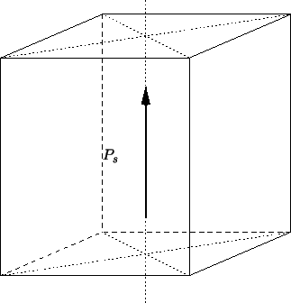
Depending on the temperature there are two other distorted crystal
phases for
![]() , each of them with a different geometry
of the unit cell. For temperatures beyond
, each of them with a different geometry
of the unit cell. For temperatures beyond ![]() C the crystal
becomes rhombohedral, between
C the crystal
becomes rhombohedral, between ![]() C and about
C and about ![]() C
monoclinic. This will raise different orientations and absolute
values of the spontaneous polarization [Kit86]. The respective unit
cells are sketched in Fig. 2.7 and Fig. 2.8.
C
monoclinic. This will raise different orientations and absolute
values of the spontaneous polarization [Kit86]. The respective unit
cells are sketched in Fig. 2.7 and Fig. 2.8.
Initially, all the spontaneous polarizations of individual cells will be randomly distributed throughout the material, so the resulting overall displacement will be zero.
If an electric field is applied, the ions will be pushed towards the
energetically better position, and if the applied field is big enough, the
ions will cross the potential barrier. In an undistorted, perfect
crystal this transition field is the same for each lattice
cell. Impurities and stress modify the energy barriers locally and
smoothen the resulting ![]() characteristics.
characteristics.
When all the dipoles are organized into the same direction, the maximum
contribution of the dipole moment to the displacement is
reached. This component is called saturation
polarization
![]() .
.
If the electric field is reduced to zero again, many of the dipoles
will be trapped in the last state causing a resulting polarization of
the material, called remanent polarization
![]() . If
the electric field is turned into the other direction, the resulting
polarization is decreased to zero. The field necessary to achieve this
is called the coercive field
. If
the electric field is turned into the other direction, the resulting
polarization is decreased to zero. The field necessary to achieve this
is called the coercive field ![]() . This behavior leads to a
hysteresis of the
. This behavior leads to a
hysteresis of the ![]() characteristics, outlined in
Fig. 2.9. The effects related to hysteresis can be summarized as follows:
characteristics, outlined in
Fig. 2.9. The effects related to hysteresis can be summarized as follows:
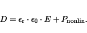
Similar to magnetism the ![]() characteristics can be separated into a linear
and a nonlinear part,
characteristics can be separated into a linear
and a nonlinear part,
Even though wrong from a rigorous point of view, it
has become quite common in the literature on ferroelectrics to denote the
nonlinear part
![]() as polarization. As the nonlinear part stems from
the switching dipoles, it will be denoted as
as polarization. As the nonlinear part stems from
the switching dipoles, it will be denoted as
![]() throughout this
work.
throughout this
work.
![\resizebox{\halflength}{!}{
\includegraphics[width=\halflength]{figs/potential_well_img.eps}
}](img123.gif)
![\resizebox{\halflength}{!}{
\psfrag{Ps}{$P_s$}
\includegraphics[width=\halflength]{figs/rhombo.eps}
}](img126.gif)
![\resizebox{\halflength}{!}{
\psfrag{Ps}{$P_s$}
\includegraphics[width=\halflength]{figs/monocl.eps}
}](img127.gif)
![\resizebox{12cm}{!}{
\psfrag{E}{$E$}
\psfrag{P}{$P_\mathrm{nonlin}$}
\psfrag{Ec}...
...}$}
\psfrag{Prem}{$P_\mathrm{Rem}$}
\includegraphics[width=12cm]{figs/Sat.eps}
}](img129.gif)