 , at time T using the Wigner function:
The computational task at hand is to calculate the statistical mean of an arbitrary physical quantity, represented by A, at time T using the Wigner function:
 = δ
= δ ).
).
It is formally proven in [117] that a linear functional of the form (3.25) can be solved by calculating the statistical expectation value of a random variable, which is calculated using the procedure discussed in Section 3.5.
The RHS of (3.18) represents an inner product between gi and f, which is reminiscent of the inner product (3.25). Therefore, either f or g can be solved to obtain the mean value of a physical quantity. In the latter case the free term gi of the adjoint equation (3.17) is chosen to correspond to the physical quantity A, augmented with the time variable, such that:
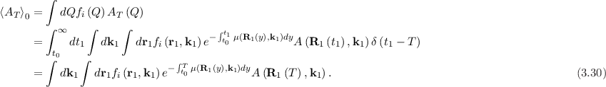
The statistical mean of AT can be expressed as:
which can be developed into a Neumann series of the formThe first expansion of g as a Fredholm equation, with the free term (3.26) yields:

 follows a trajectory R1 and reaches the point
  with a probability of
e-∫
t0Tμ
with a probability of
e-∫
t0Tμ dy and makes a contribution of A
 to the statistical mean of A. If the particle is scattered from its trajectory, it contributes through
another term in the series.
to the statistical mean of A. If the particle is scattered from its trajectory, it contributes through
another term in the series.
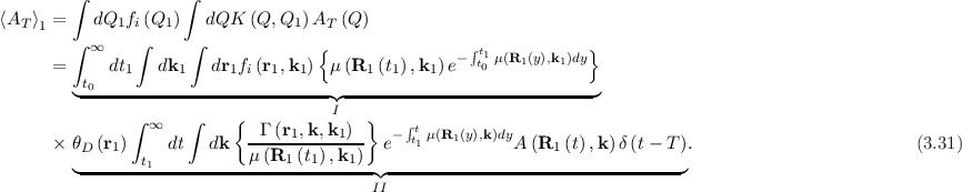
 follows a trajectory R1, but only until time t1 where it is scattered. By extracting μ as a common factor, the
term in the first set of braces can be interpreted as the probability for a particle to not be scattered until time t1 (the exponential) and then
to be scattered in the interval dt1 thereafter
follows a trajectory R1, but only until time t1 where it is scattered. By extracting μ as a common factor, the
term in the first set of braces can be interpreted as the probability for a particle to not be scattered until time t1 (the exponential) and then
to be scattered in the interval dt1 thereafter  . The term in the braces of term II describes the probability of scattering
from k1 to k and the exponential term again gives the probability that the scattered particle will not be scattered again until time T, where it
contributes A
. The term in the braces of term II describes the probability of scattering
from k1 to k and the exponential term again gives the probability that the scattered particle will not be scattered again until time T, where it
contributes A to the statistical mean of A. If the particle is scattered again before time T, it contributes through another term in the
series.
to the statistical mean of A. If the particle is scattered again before time T, it contributes through another term in the
series.
Further terms of the series can be written down in a similar manner to reveal the general structure: A particle that scatters n times before time T makes a
contribution to  through the term
  n in the series. The braced terms in the integrals of I and II represent probabilities, which clearly establishes the link to
the Monte Carlo integration introduced in Section 3.5.
n in the series. The braced terms in the integrals of I and II represent probabilities, which clearly establishes the link to
the Monte Carlo integration introduced in Section 3.5.
The term  appearing in term II represents the total scattering probability, including both phonons and the ’scattering’ (particle generation) associated to
the Wigner potential. Phonon scattering occurs with a probability
appearing in term II represents the total scattering probability, including both phonons and the ’scattering’ (particle generation) associated to
the Wigner potential. Phonon scattering occurs with a probability  and is described in Section 3.7.5; the Wigner-related term is selected with a probability
 =
=  and can then be written as
Two interpretations of (3.32) are possible: If considered as a scattering mechanism, one of the terms is selected, each with a probability 1∕3 and the particle is generated with a weight of ±3 at wavevector ±k′. Alternatively, all three terms can be chosen simultaneously and take a weight of ±1, i.e. two additional particles are created with wavevector ±k′ and weight ±1; the original particle, associated with the δ, persists unchanged. The algorithm to select the wavevectors of the generated particles is discussed in Section 3.7 and revisited in Chapter 4, which considers the semi-discrete form of the WBE.


