Subsections

• 6.6.1 Interface Degradation
• 6.6.2 Drift-Diffusion
• 6.6.3 Trapping

6.6 The New Model for Numerical Simulation of NBTI

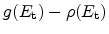
Figure 6.16: Schematic illustration of the model as implemented in Minimos-NT giving an overview of the involved processes.

From literature it is obvious that no clear consensus about the physical mechanism nor a model which is commonly agreed upon is found up to now. Various research groups report different key mechanisms leading to NBTI and therefore propose different models which sometimes completely contradict each other [85,110,102,86,122]. Is it purely the interface degradation, are oxide traps or oxide charges involved, is hole trapping important, are Si-H or also Si-O bonds broken et cetera.

In this section a model is proposed which was implemented into the numerical device simulator Minimos-NT. Figure 6.16 gives an overview of the involved processes. The model is able to achieve excellent agreement with measurement data on thick, pure dielectrics of high-voltage devices from our industry partner (Section 7.1) for both, the stress and the relaxation phase of NBTI and for different temperatures.

As the model comprises of many models and physical assumptions described in different parts of this work, I will collect all important equations in this section for the sake of clarity.

6.6.1 Interface Degradation

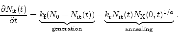
The first mechanism is the interface degradation as proposed in the reaction-diffusion model (Section 6.4). It is described in form of a balance equation between generation of electrically active interface traps ( ) due to a forward term, and interface trap annealing as a result of a backward term as follows

$$\frac{\partial \ensuremath{N_\textrm{it}}(t)}{\partial t} = ... ...ensuremath{N_\textrm{X}}(0,t)^{1/a}}_{\mathrm{annealing}} .$$ (6.31)

The important parameters in this equation are the forward reaction rate, , the sum of passivated and broken interface states , the reverse reaction rate , the amount of the mobile species directly available at the interface, and the kinetics exponent, $a$, giving the type of mobile species.

Assuming electrically neutral hydrogen, , or hydrogen protons, , the kinetics exponent $a$ equals $1$. In this case, for every generated a mobile hydrogen, , is released. To assume molecular hydrogen, , as the mobile species the kinetics exponent equals $2$.

The amount of interface states is strongly dependent on the wafer orientation and the process technology. It can greatly differ for different interfaces. Reasonable values are often in the range of $10^{12}$-$10^{14}$cm$^{-2}$ as described in Section 3.1. For reliable device operation it is, of course, of highest interest to keep this number as low as possible.

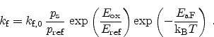
The forward reaction rate is dependent on the local electric field, , and the local hole concentration

$$\ensuremath {k_\textrm{f}}= \ensuremath{k_\textrm{f,0}} \f... ...extrm{aF}}}{\ensuremath{\textrm{k$_\textrm{B}$}}T}\right) .$$ (6.32)

Here, is the Boltzmann constant and $T$ the temperature. The prefactor , the reference hole concentration , and the reference electric field are model calibration parameters. The temperature dependence is introduced by an Arrhenius' law of the activation energy , which is also a calibration parameter. The influence of the electric field in this equation is exponential and change in the field has therefore a major impact on the forward reaction rate while the hole concentration has only little impact in agreement with experimental observations [101].

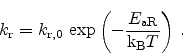
The reverse reaction rate is also introduced as Arrhenius activated with the activation energy and the prefactor

$$\ensuremath{k_\textrm{r}}= \ensuremath{k_\textrm{r,0}} \e... ...extrm{aR}}}{\ensuremath{\textrm{k$_\textrm{B}$}}T}\right) .$$ (6.33)

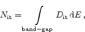
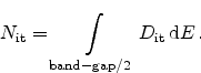
As described in Section 3.1, the energy distribution of electrically active interface traps can be very important. When the Fermi-level is not very close to one of the band edges, the charge state of these traps differs depending on their density-of-states (DOS). The density of is given as the integral of across the whole band-gap

$$\ensuremath{N_\textrm{it}}= \int_\mathrm{band-gap} \ensuremath{D_\textrm{it}} \mathrm{d}E ,$$ (6.34)

or, when considering the amphoteric nature of the traps with their double peaks (Section 3.1.1)

$$\ensuremath{N_\textrm{it}}= \int_{\mathrm{band-gap}/2} \ensuremath{D_\textrm{it}} \mathrm{d}E .$$ (6.35)

Several models for different DOS are available in Minimos-NT, where the most plausible according to literature are two peaks of Gaussian form as found in Section 3.1.2.

6.6.2 Drift-Diffusion

The next mechanism in the degradation process is the (drift-) diffusion of the hydrogen related species from the interface into the dielectric.

The convection of the electrically neutral species and is a purely diffusive process due to the concentration gradient

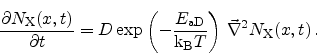$$\frac{\partial \ensuremath{N_\textrm{X}}(x,t)}{\partial t} ... ...uremath{{\vec{\nabla}}}^2 \ensuremath{N_\textrm{X}}(x,t) .$$ (6.36)

Here, $D$ is the diffusion constant. The temperature dependence was introduced using Arrhenius' law with the activation energy .

For the case of proton transport, , an additional drift term has to be added to (6.36). In the typical NBT stress condition where a negative voltage is applied to the gate contact, this leads to quick removal of the positively charged protons from the interface. As a consequence more interface traps can break and the degradation is increased.

6.6.3 Trapping

To account for the dispersive transport theory as described in Section 6.4.3, the trapping and de-trapping of the mobile species in the dielectric is included in this model.

At each trap center in the dielectric a balance equation is solved to account for the trapping and de-trapping effects. The trap occupancy $\rho(\ensuremath{E_\textrm{t}})$ is considered at each trap energy level as

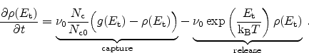$$\frac{\partial \rho(\ensuremath{E_\textrm{t}})}{\partial t}... ...\right) \rho(\ensuremath{E_\textrm{t}})}_\mathrm{release} .$$ (6.37)

Here, is the hydrogen effective density-of-states, the release rate coefficient, the amount of available, uncaptured hydrogen and $g(\ensuremath{E_\textrm{t}})$ the trap density-of-states at this energy level. In the capture part of this equation the filling of traps is accounted for ( $g(\ensuremath{E_\textrm{t}}) - \rho(\ensuremath{E_\textrm{t}})$) so that the maximum possible amount of trapped hydrogen at each trap level equals the DOS. The release of hydrogen is dependent on the ``depth'' of the trap. Deeper traps have an exponential decrease in their de-trapping probability.

The trap energy is zero at the mobility edge and below zero at the trap levels with more negative values for deeper traps. Therefore, with decreasing temperature the trap release rate decreases ( $\exp(\ensuremath{E_\textrm{t}}/\ensuremath{\textrm{k$_\textrm{B}$}}T)$) and de-trapping becomes more unlikely. The trapping probability does not change in this model.

Within the model the charge state of trapped hydrogen can be chosen to model the formation of positively charged trapped protons, as described in [107].

The DOS of the trap levels can be selected from the model. Two plausible densities are schematically illustrated on the right hand side of Figure 6.16. An exponential distribution with the highest DOS at the band edge [88] or with an additional Gaussian peak in deeper states forming deep and therefore ``slow'' traps [106,107,108].

Table 6.1: NBTI model parameters.

Parameter	Unit	Description
	cm$^{-2}$	Total density of interface states (el. active and inactive)
$a$	1	Kinetics exponent automatically set according to diffusing species
	s$^{-1}$	Forward reaction rate prefactor
	cm$^{-3}$	Reference hole concentration
	V cm$^{-1}$	Reference electric field
	eV	Forward reaction activation energy
	cm$^3$ s$^{-1}$	Reverse reaction rate prefactor
	eV	Reverse reaction activation energy
$D$	cm$^2$ s$^{-1}$	Diffusion coefficient
	eV	Diffusion activation energy
	cm$^{-3}$	Hydrogen effective density-of-states
	s$^{-1}$	Trapping/de-trapping frequency