


Next: 6.5 Tsetseris' Model
Up: 6. Negative Bias Temperature
Previous: 6.3 Physical Mechanisms of
Subsections
6.4 Reaction-Diffusion Model
Figure 6.10:
Schematic representation of the reaction-diffusion (R-D) model.
Electrically inactive Si-H bonds at the
 interface are broken and the
hydrogen diffuses into the dielectric leaving behind an electrically active
interface trap
interface are broken and the
hydrogen diffuses into the dielectric leaving behind an electrically active
interface trap
 . Here, H
 diffusion is assumed.
|
|
The reaction-diffusion (R-D) model is pioneering for the description of NBTI.
It was first proposed by Jeppson and Svensson in 1977 [103] and is
capable of reproducing the time evolution of device degradation due to negative
bias temperature stress for a wide range of measurements.
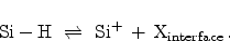
The model describes the device degradation as a combination of two effects. In
the first place, a field-dependent electrochemical reaction at the
interface. Electrically inactive, passivated silicon dangling bonds
(Section 3.1), Si-H, are broken. Here an electrically
active interface state
and a mobile, hydrogen related species
 are
formed,
are
formed,
 |
(6.5) |
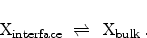
In the second place, the model describes the transport of the hydrogen species
away from the interface into the dielectric,
 |
(6.6) |
Also the reverse process is possible: transport of a diffusing hydrogen species
back to the interface and re-passivation of a
 dangling bond.
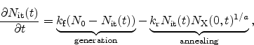
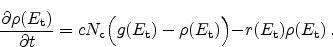
Figure 6.10 gives a schematic illustration of the model. In the
figure hydrogen molecules,
 , are assumed as the diffusing species. The
process at the interface is modeled by a rate equation as
, are assumed as the diffusing species. The
process at the interface is modeled by a rate equation as
 |
(6.7) |
where
 is the interface-trap generation and
 the annealing rate. The
symbol
the annealing rate. The
symbol
 denotes the initial number of electrically inactive Si-H bonds and
 is the surface concentration of the diffusing species. The value of
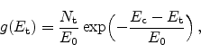
 gives the order of the reaction. In the original publication, neutral
hydrogen, H
gives the order of the reaction. In the original publication, neutral
hydrogen, H , was proposed [103] which is obtained with
  .
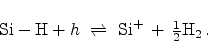
For molecular hydrogen,
,
.
For molecular hydrogen,
,  . In this case the molecule is assumed
to be formed in the vicinity of the interface
. In this case the molecule is assumed
to be formed in the vicinity of the interface
 |
(6.8) |
The Si-H bond is broken and captures a hole, leading to a positively charged
interface state and molecular hydrogen is formed.
The equilibrium of the forward and backward reaction is controlled by the
hydrogen density at the interface
. Thus, the transport mechanism of
the hydrogen species away from the interface characterizes the degradation
mechanism, controlling the device parameter shift. The original
reaction-diffusion model describes the transport as a purely diffusive
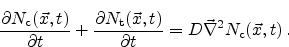
mechanism which is described by the diffusion equation
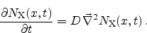 |
(6.9) |
Here,  is the diffusivity of the hydrogen species in the dielectric. The
influx of the newly created species has to be considered as
is the diffusivity of the hydrogen species in the dielectric. The
influx of the newly created species has to be considered as
 |
(6.10) |
For each generated interface trap a hydrogen is released, thus
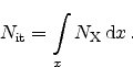 |
(6.11) |
The R-D model assumes the interface states to be the only contribution to
device parameter shift. But especially thick high-voltage oxides also show the
generation of oxide charges due to hole trapping [86], leading to an
additional parameter shift. Therefore it has been suggested [85] to
separate the oxide charge contribution from the measurement results, before the
R-D model can put into agreement to them. Suggested methods are the estimation
of bulk-trap concentration for every stress voltage, temperature, and oxide
thickness or trying to avoid the generation of bulk-traps by optimizing the
stress conditions to that aspect.
Figure 6.11:
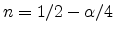
The five different regimes for the time exponent  , as obtained
from the reaction-diffusion model.
, as obtained
from the reaction-diffusion model.
|
|
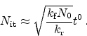
For the stress phase the solution of the R-D model can be split up into five
different regimes. They are distinguished by different time exponents
(Section 6.2) for the degradation and are depicted in
Figure 6.11.
In the very early stage of the stress phase the amount of free hydrogen, both,
at the interface and in the dielectric
 is very low. The amount of
already broken Si-H bonds at the interface
is close to zero. Thus,
Equation 6.7 is solely limited by the forward reaction rate
and
transforms to
is very low. The amount of
already broken Si-H bonds at the interface
is close to zero. Thus,
Equation 6.7 is solely limited by the forward reaction rate
and
transforms to
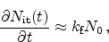 |
(6.12) |
with the solution for the interface trap generation
 |
(6.13) |
when assuming
 |
(6.14) |
having a time dependence of  .
.
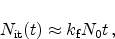
After some time, when the amount of hydrogen at the interface is considerable,
the forward reaction reaches a quasi-equilibrium with the backward reaction
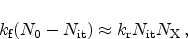 |
(6.15) |
and, as
is very large with respect to
 |
(6.16) |
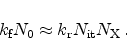
The diffusion process has not removed a considerable amount of hydrogen from
the interface yet, therefore the amount of interface traps equals the amount of
hydrogen at the interface
 |
(6.17) |
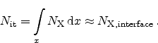
We therefore get
 |
(6.18) |
As this equation is not time dependent we can write
 |
(6.19) |
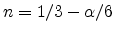
with a resulting time dependence of  .
.
As long as the diffusion of hydrogen away from the interface has not reached a
considerable magnitude, there is no further degradation of the interface.
Regime three starts when the diffusion of hydrogen away from the interface sets
in and acts as limiting factor for the degradation. In this phase the
diffusion front has not reached the poly gate, therefore
 |
(6.20) |
An analytical solution has been found to be [103]
 |
(6.21) |
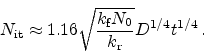
Numerically the solution is, depending on the group, somewhat
larger [85] or smaller [104] then the analytical
solution of  as it is based on some simplifications.
In the reaction-diffusion model, this is the dominating regime in the typical
lifetime of a MOSFET. It sets in after some seconds stress and, depending on
the exact conditions, is dominating for several orders of magnitude in time,
lasting up to several years.
When the diffusion front reaches the poly gate contact the time exponent
changes again. In the model it is assumed that the gate electrode acts as
absorber for the diffusing species or, in other words, the diffusivity is
significantly higher in the poly than in the dielectric. For this case a time
exponent of  is derived. Although a slight increase of the time
exponent can be found in some measurement data for thin dielectrics, it is way
below
is derived. Although a slight increase of the time
exponent can be found in some measurement data for thin dielectrics, it is way
below  .
.
When, theoretically, all interface bonds
are broken and
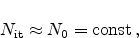 |
(6.22) |
no further degradation can occur in this model. Therefore the change in
is zero and so is the time exponent . As this saturation condition would
only occur ever at extremely long stress times, or, at very high stress
conditions which would lead to other degradation mechanisms as TDDB
(Section 5.2), it has not yet been observed experimentally.
It has been shown that the measured degradation and also the extracted time
exponent strongly depend on the time delay during measurement. Using fast
measurement methods to spot the full degradation during NBT stress reveals a
very low time exponent around 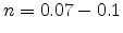 (see Section 6.3.6). The
reaction-diffusion model, in contrast, predicts a time exponent of for
neutral hydrogen diffusion,
(see Section 6.3.6). The
reaction-diffusion model, in contrast, predicts a time exponent of for
neutral hydrogen diffusion,
 . By assuming molecular hydrogen being the
diffusing species a time exponent of
. By assuming molecular hydrogen being the
diffusing species a time exponent of  can be achieved. Here, an
additional reaction step at the interface generates molecular hydrogen before
diffusion,
can be achieved. Here, an
additional reaction step at the interface generates molecular hydrogen before
diffusion,
 . Only by introducing higher order
chemical reactions at the interface the time exponent could be further reduced
to fit the model to state-of-the-art measurement results.
. Only by introducing higher order
chemical reactions at the interface the time exponent could be further reduced
to fit the model to state-of-the-art measurement results.
The fast recovery effect poses another inconsistency of the pure R-D model with
measurement data [99]. Even for very long stress times of more than
1000 seconds the immediate recovery of
 in the first second after stress
is more than 60% using the fast measurement set-up.
in the first second after stress
is more than 60% using the fast measurement set-up.
Figure 6.12:
Hydrogen profiles in the dielectric for 1000 second stress (left)
and after the recovery of 60 % of the degradation. It is difficult to
argue that the diffusion of more than half of the hydrogen which took 1000
seconds to diffuse into the dielectric can diffuse back to the interface in
one second [99].
|
|
The R-D model assumes diffusion limited degradation and also diffusion limited
relaxation. When considering a stress time of 1000 seconds a certain amount of
hydrogen related species diffuses into the dielectric as shown in
Figure 6.12. The total amount of hydrogen in the dielectric must equal
the number of interface traps
(6.11).
is in turn
directly proportional to the shift of the threshold voltage
 . To argue
a 60% recovery during the first second in the framework of the R-D model,
60% of the hydrogen must diffuse back to the interface and anneal the
dangling silicon bonds within this second. This would result in a hydrogen
profile in the dielectric, as seen on the right hand side of
Figure 6.12, implying that the backward diffusion must be orders of
magnitude faster than the forward diffusion [99].
. To argue
a 60% recovery during the first second in the framework of the R-D model,
60% of the hydrogen must diffuse back to the interface and anneal the
dangling silicon bonds within this second. This would result in a hydrogen
profile in the dielectric, as seen on the right hand side of
Figure 6.12, implying that the backward diffusion must be orders of
magnitude faster than the forward diffusion [99].
6.4.3 Dispersive Transport
Figure 6.13:
Schematic illustration of dispersive transport. Hydrogen is
dissociated from the interface and transported into the
 via a
diffusive mechanism. In the dielectric the mobile species sees traps of
different energies leading to dispersive transport. The energy diagram on
the right hand side shows a possible density-of-states (DOS) energy
distribution of the traps.
via a
diffusive mechanism. In the dielectric the mobile species sees traps of
different energies leading to dispersive transport. The energy diagram on
the right hand side shows a possible density-of-states (DOS) energy
distribution of the traps.
|
|
Instead of using the standard diffusion equation [103,105] to
describe hydrogen transport in the dielectric it has been
shown [88,106,107,108,109,110,111,112]
that correct modeling of transport in an amorphous materials must consider its
dispersive [113] nature.
Figure 6.14:
At small times the energy distribution of trapped carriers is
similar to the density-of-states (DOS) as the trapping probability for each
trap is the same. After time the peak of the energy distribution moves
towards deeper states. The reason is the higher de-trapping probability for
shallow traps.
|
|
Dispersion arises when the mobile species experiences different barrier heights
at different positions in space. Figure 6.13 gives a schematic
illustration where the dielectric contains hydrogen traps of different energy.
The trapping probability at each trap is the same. But for de-trapping the
deeper traps pose a higher barrier than the shallow ones. This implies that at
the beginning of the trapping events the energy distribution of trapped
carriers is proportional to the density-of-states (DOS). But after some time,
as de-trapping preferably occurs for shallow traps, the peak of the energy
distribution moves to deeper traps as illustrated in
Figure 6.14. Thus, the equilibrium distribution is totally
different from the DOS.
In the modeling approach, the species
is separated into two distinct
contributions. The conducting,
 , and trapped,
 , particles. The
trapped particles are distributed in energy where the density at a trap
energy-level
, particles. The
trapped particles are distributed in energy where the density at a trap
energy-level
 is given as
 . The trapped particles do not
contribute to the transport. To introduce dispersive transport into the
reaction-diffusion model, (6.9) transforms to
. The trapped particles do not
contribute to the transport. To introduce dispersive transport into the
reaction-diffusion model, (6.9) transforms to
 |
(6.23) |
At each trap energy-level a rate equation describes the dynamics between
trapping and de-trapping as
 |
(6.24) |
Here,  is the capture rate,
 the energy-dependent release rate,
and
the energy-dependent release rate,
and
 is the trap DOS.
When considering the trap distribution in exponential
form [113,92]
 |
(6.25) |
and with introduction of the dispersion parameter
 |
(6.26) |
can, for neutral species, be expressed with a power-law
as [114]:
 |
(6.27) |
with
 being the release rate coefficient. Here, only hydrogen in the
conductive state can contribute to the reverse rate.
being the release rate coefficient. Here, only hydrogen in the
conductive state can contribute to the reverse rate.
When assuming atomic hydrogen () the slope calculates from
(6.27) as
 while when assuming molecular hydrogen
()
results in
while when assuming molecular hydrogen
()
results in
 . In both cases the time exponent
is increasing for an increasing dispersion parameter
. In both cases the time exponent
is increasing for an increasing dispersion parameter  . So for an
increasing number of deep traps the degradation
increases [104,111].
. So for an
increasing number of deep traps the degradation
increases [104,111].
For complex trap distribution functions no analytic formulation can be found.
An example is a combination of shallow band-tail traps (the exponential
distribution) and deep Gaussian traps describing deep traps (right hand side of
Figure 6.13) [111]. For such a DOS only the
numerical solution is possible as obtained with the numerical device simulator
Minimos-NT.
6.4.4 Coupling to the Semiconductor Device Equations
As NBTI is strongly dependent on the stress conditions, the available models
include at least the dependence on the electric field (the bias) and the
temperature. But also the hole concentration at the interface might be of
interest [85].
In the one-dimensional NBTI models the values of these quantities are accounted
for in the model parameters, as
and
in the reaction-diffusion model
for example. For each device, stress voltage, and temperature these parameters
are extracted (Section 7.1.2) and are assumed constant for these
stress conditions. But as degradation is continuing during stress, the
underlying parameters, especially the electric field across the interface,
change. So the electric field at the
interface is decreasing when the
NBTI induced degradation leads to positive charge build up at this interface.
Therefore, it might not be appropriate to consider the forward reaction rate
as a constant.
Another point is the two-, or three-dimensional investigation of a device
structure. Here the electric field and the hole concentration, and therefore
also the magnitude of degradation, can change drastically across the channel of
the device when the stress conditions are not uniform
(Section 6.3.3). Thus, the model parameters are not uniformly
distributed at the
interface and a one-dimensional consideration of
the model might not be accurate enough [115].
To solve these issues it is important to include the NBTI models into a
numerical device simulation. The distributed quantities, obtained from the
semiconductor device equations (Section 2.1) as the electric
field, hole and electron concentration can be directly used in the degradation
model. The resulting charge densities from the NBTI model can be included in
the device equation leading to a fully self-consistent coupling of those two
sets of equations.
The reaction-diffusion model might be linked to the semiconductor device
equations with the forward reaction rate as follows [85]
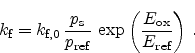 |
(6.28) |
Where
 and
and
 are the hole concentration and the electric field at the
interface,
are the hole concentration and the electric field at the
interface,
 and
and
 are reference values. By using solution
variables of the semiconductor equations the NBTI model can be applied to
arbitrary device geometries.
are reference values. By using solution
variables of the semiconductor equations the NBTI model can be applied to
arbitrary device geometries.
Next: 6.5 Tsetseris' Model
Up: 6. Negative Bias Temperature
Previous: 6.3 Physical Mechanisms of
R. Entner: Modeling and Simulation of Negative Bias Temperature Instability
![\includegraphics[width=12cm]{figures/nbti-schematic}](img521.png)
![\includegraphics[width=12cm]{figures/rd-regimes}](img541.png)
![\includegraphics[width=16cm]{figures/rd-vs-fast}](img563.png)
![\includegraphics[width=16cm]{figures/nbti-dispersive-transport-gauss}](img564.png)
![\includegraphics[width=\figwidth]{figures/sg-trapping}](img565.png)