6.5 Focused Ion Beam Processing

Another application of the presented simulation techniques are FIB simulations. So far, full three-dimensional simulations have been presented in [55] and [57] using cell- and segment-based methods for surface evolution, respectively. The application of the LS method for FIB simulations was first demonstrated in [58]; however, only for the two-dimensional case. In this section, three-dimensional FIB simulations using the LS method and ray tracing are presented.

The same model is used as described in [57], which also considers redeposition of sputtered material. Sputtered particles are assumed to remain sticking with a probability ${s}=1$ . The surface velocity is given by the difference of the sputter rate and the deposition rate of redeposited particles. Here, the sputter rate is modeled using Yamamura's formula (2.21). There, the constants ${C}_1$ and ${C}_2$ are chosen in such a way that the maximum sputter rate is 20 particles per ion for an incident angle of $\SI{82}{\degree}$ . For normal incidence a sputter rate of 2.5 is assumed. The directions of sputtered particles are described by a cosine distribution (2.19). The beam profile is modeled using a normal distribution (2.11).

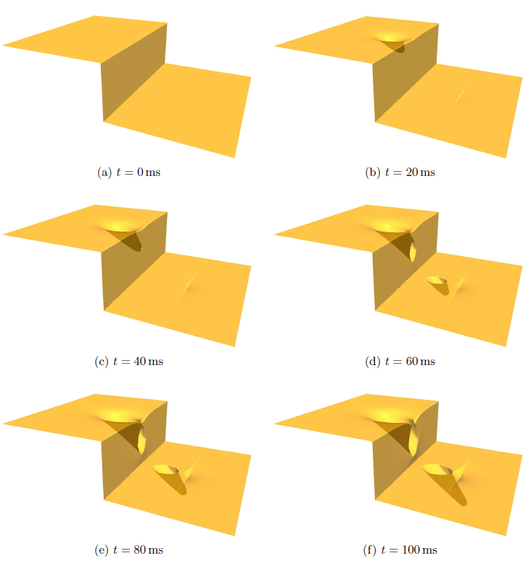
The first example (Figure 6.12) shows the effect of an ion beam with diameter $\SI{50}{\nano\metre}$ (FWHM) and inclined incidence with angle $\SI {45}{\degree }$ on a step structure. The LS method is able to describe the appearing topographic changes without any problems. The beam current is set to $\SI{50}{\pico\ampere}$ and the bulk density is assumed to be that of silicon ( ${\rho}_{\text{Si}}=\SI{5e28}{\per\cubic\metre}$ ). The grid spacing is set to $\SI{2}{\nano\metre}$ . One million ions are launched at every time step in order to calculate the surface velocities.

Figure 6.12: Ion beam milling of a step structure for an incident angle of $\SI {45}{\degree }$ .

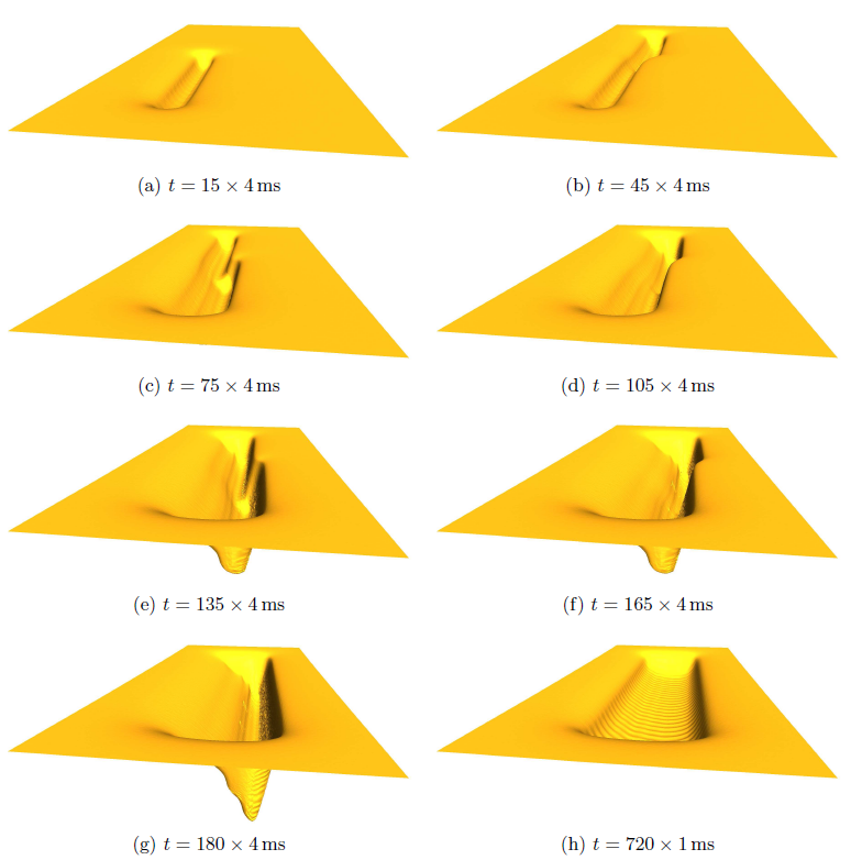
As a second example, the time evolution of a plain surface, which is processed by a normal incident FIB as described in [57], is calculated. The beam is moved over $30\times 6$ pixels using a serpentine scan strategy. The overlap of two neighboring pixels is assumed to be $\SI{50}{\percent}$ , which means that the distance between their midpoints is $\SI{50}{\percent}$ of the beam diameter, thus $\SI{25}{\nano\metre}$ . Figure 6.13 shows the results for two different processing schemes: a single pass with a dwell time of $\SI {4}{\milli \second }$ at every pixel and four passes with a dwell time of $\SI {1}{\milli \second }$ .

Figure 6.13: (a)-(g) Serpentine scan of $30\times 6$ pixels with dwell time of $\SI {4}{\milli \second }$ . (h) Four passes of a serpentine scan with dwell time of $\SI {1}{\milli \second }$ .