


Next: 3.3.2 Curvature
Up: 3.3 Approximations to Geometric
Previous: 3.3 Approximations to Geometric
3.3.1 Surface Normal
Generally, the normal vector at point  on the LS of a smooth function is given by
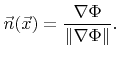 |
(3.21) |
At grid points
 the
the  -th component of the normal vector can be approximated by
 |
(3.22) |
Here  is the central difference operator as defined in (3.6).
The normal vector for a grid point close to the surface
is the central difference operator as defined in (3.6).
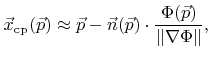
The normal vector for a grid point close to the surface
 represented by the zero LS is also a good approximation for the normal on the surface for the closest surface point. The closest surface point
 of a nearby grid point
  can be approximated by [135]
 |
(3.23) |
if the grid point indices
are equal to the grid point coordinates. Here the last factor corresponds to the approximated signed distance to the surface. For the denominator the same approximation is used as in (3.22).
Next: 3.3.2 Curvature
Up: 3.3 Approximations to Geometric
Previous: 3.3 Approximations to Geometric
Otmar Ertl: Numerical Methods for Topography Simulation