3.3.2 Curvature

Solving the LS equation with a velocity field that is proportional to the curvature can be used for smoothing as will be demonstrated in Section 4.5. For an arbitrary point ${\vec{x}}$ the (mean) curvature of the corresponding LS is defined as

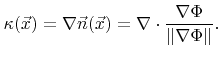$${\kappa}({\vec{x}})=\nabla{\vec{n}}({\vec{x}})=\nabla\cdot\frac{\nabla{{\Phi}}}{\lVert\nabla{{\Phi}}\rVert}.$$ (3.24)

At grid points ${\vec{p}}\in{\mathcal{G}}$ the mean curvature can be approximated by [110]

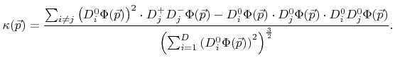$${\kappa}({\vec{p}}) = \frac{\sum_{i\neq j} \left({D}_{i}^{0}{\Phi... ...ft(\sum_{i=1}^{D}\left({D}^0_{i}{\Phi}({\vec{p}})\right)^2\right)^\frac{3}{2}}.$$ (3.25)