To reduce the number of hierarchical traversals within a tree, direct neighbor links to subboxes have been proposed [72]. Apart from single neighbor links between nodes at the same level of the kd-tree, neighbor links trees can be used [39] to link leaves which correspond to subboxes, directly. A tree is set up for each face of a subbox to enable direct traversals to neighboring subboxes. Hence, using the exit point the next traversed subbox can be obtained by querying the corresponding neighbor links tree.

|
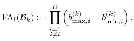
In the following discussion a new neighbor links data structure is presented. Using the fact that splitting planes are always aligned with the grid, arrays can be used to store the links to neighbor boxes, as demonstrated for a two-dimensional example in Figure 5.4. The number of links which are required for box
![]() , is equal to its surface area
, is equal to its surface area
![]() (measured in grid spacings).
(measured in grid spacings). ![]() different arrays
different arrays
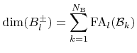
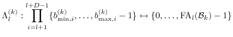
![]() hold the neighbor links in a certain grid direction for all boxes. The number of links is equal for opposite directions. Hence, for each box
hold the neighbor links in a certain grid direction for all boxes. The number of links is equal for opposite directions. Hence, for each box
![]() only
only ![]() array indices
array indices
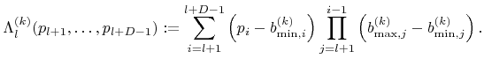
![]() have to be stored in order to obtain the corresponding neighbor links. The size of the array
have to be stored in order to obtain the corresponding neighbor links. The size of the array ![]() is given by
is given by
 |
(5.26) |
![$\displaystyle {B}_l^\pm \left[ {i}_l^{(k)}+{\Lambda}_l^{(k)}(\lfloor{x}_{l+1}\rfloor,\ldots,\lfloor{x}_{l+{D}-1}\rfloor) \right].$](img679.png) |
(5.27) |
 |
(5.28) |
 |
(5.29) |
Additional links from outside of
![]() allow finding the box which must be traversed first. They are stored in the
allow finding the box which must be traversed first. They are stored in the ![]() arrays
arrays
![]() with size
with size
| (5.31) |
 |
(5.32) |
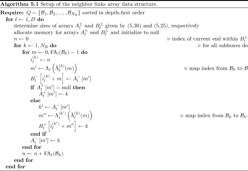
Once an appropriate spatial subdivision is found for
![]() , the neighbor links data structure can be set up. For subdivisions which are obtained by binary splitting in depth-first order, the neighbor links arrays data structure can be set up in optimal time (directly proportional to the total memory requirements) using Algorithm 5.1.
, the neighbor links data structure can be set up. For subdivisions which are obtained by binary splitting in depth-first order, the neighbor links arrays data structure can be set up in optimal time (directly proportional to the total memory requirements) using Algorithm 5.1.
The neighbor links data structure allows an easy treatment of periodic boundary conditions. The boxes which are situated at the boundary can be directly linked to the corresponding boxes at the opposite boundary.