Another MC technique, which can be used to calculate the surface rates directly, is ray tracing [10,114]. Ray tracing is a widely applied technique in computer graphics for rendering a scene. A large number of light rays is used to obtain a realistic picture. In recent years, this MC technique has been successfully applied to topography simulation to calculate surface rates [8,64,95]. Especially if the particle trajectories are linear, which is the case for ballistic transport, the same algorithms and techniques can be applied in an analogous manner [A13,A16].
In order to simulate the particle transport and to obtain the surface rates, many particles are launched from the source plane
![]() , and their trajectories are calculated. Whenever a particle reaches the surface
, and their trajectories are calculated. Whenever a particle reaches the surface
![]() , it contributes directly to the local surface rates introduced in (2.24). For each surface point
, it contributes directly to the local surface rates introduced in (2.24). For each surface point ![]() , for which the rates should be calculated, a surrounding neighborhood is defined. If the area of that neighborhood, denoted by
, for which the rates should be calculated, a surrounding neighborhood is defined. If the area of that neighborhood, denoted by
![]() , is small enough and the surface is smooth, the neighborhood can be assumed to be plane and orthogonal to the surface normal
, is small enough and the surface is smooth, the neighborhood can be assumed to be plane and orthogonal to the surface normal
![]() . These neighborhoods of known area are necessary to relate the contribution of a single particle to the rates at point
. These neighborhoods of known area are necessary to relate the contribution of a single particle to the rates at point ![]() . An incident particle of type
. An incident particle of type
![]() with direction
with direction
![]() and energy
and energy
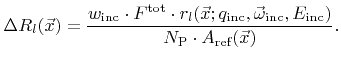
![]() striking the neighborhood of point
striking the neighborhood of point ![]() adds
adds
 |
(5.13) |
 |
(5.14) |
A better strategy is to introduce a volume or weight factor ![]() assigned to a particle as proposed in [118] and which allows to control the number of reemitted particles. Initially, when a particle is launched from the source, its weight factor is set to unity (
assigned to a particle as proposed in [118] and which allows to control the number of reemitted particles. Initially, when a particle is launched from the source, its weight factor is set to unity (![]() ). An incident particle contributes to the local rates according to its current weight factor
). An incident particle contributes to the local rates according to its current weight factor
![]()
| (5.16) |
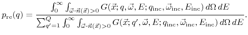
The directional and energy distribution
![]() of a reemitted particle species
of a reemitted particle species ![]() obeys
obeys
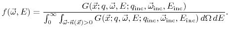 |
(5.17) |
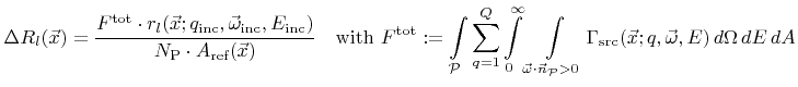
The main computational task of this ray tracing technique is to determine the first surface intersection of rays and to test for intersections with the neighborhoods of all surface points ![]() , for which the surface rates should be calculated. The choice of surface representation and of neighborhoods, as well as the corresponding intersection tests are discussed in the following sections.
, for which the surface rates should be calculated. The choice of surface representation and of neighborhoods, as well as the corresponding intersection tests are discussed in the following sections.