3.1.3 Simulating Oxide Growth using Volume Expansion

Silvaco, Inc., as mentioned in Section 3.1.1, offers a three-dimensional process simulation tool which includes empirical and mechanical oxidation simulations. Their approach to simulating the mechanics of silicon oxidation includes the use of the LS method [203]. Instead of using unstructured meshes, their approach makes use of a fixed Cartesian mesh in a LS environment, solving the problem of moving boundaries which arise when unstructured meshes are used.

The model includes four major steps which work together to generate a moving oxide interface:

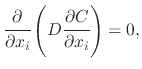
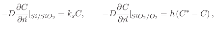
1. Oxidant diffusion through the oxide is modeled using the well-known diffusion equation

   $$\cfrac{\partial}{\partial x_{i}}\left(D\cfrac{\partial C}{\partial x_{i}}\right)=0,$$ (81)

   
   

   $$-D\cfrac{\partial C}{\partial\vec{n}}\vert _{Si\slash SiO_{2}}=k_... ...c{\partial C}{\partial\vec{n}}\vert _{SiO_{2}\slash O_{2}}=h\left(C^*-C\right),$$ (82)

   
   
   where $D$ is the diffusion coefficient, $k_s$ is the reaction rate, $h$ is the gas-phase mass-transfer coefficient, $C^*$ is the equilibrium bulk concentration in the oxide, and $\vec{n}$ is the normal to the corresponding interface. The diffusion equation is obviously identical to the one presented in Section 2.3.1.

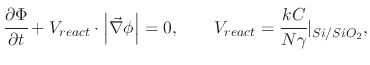
2. Propagation of the oxide-silicon interface is solved after the diffusion equation for a time step $\delta t$. To find the new position of the SiO$_2$-Si interface, the LS is solved for the distance function

   $$\cfrac{\partial\Phi}{\partial t}+V_{react}\cdot\left\vert\vec{\na... ...phi\right\vert=0,\qquad V_{react}=\cfrac{kC}{N\gamma}\vert _{Si\slash SiO_{2}},$$ (83)

   
   
   where $N$ is the number of oxidant molecules incorporated into a unit of oxide and $\gamma$ is the Si $\rightarrow$SiO$_2$ expansion coefficient. An up to third order Total Variation Diminishing (TVD) Runge-Katta scheme is used for discretization [66].

3. The volume expansion resulting from the chemical reaction is calculated using the creep equation

   $$\cfrac{\partial S_{ij}}{\partial s_{i}}=0,$$ (84)

   
   
   where $S_{ij}$ is a Cauchy stress tensor. Assuming a Maxwell visco-elastic fluid, the Cauchy stress tensor becomes

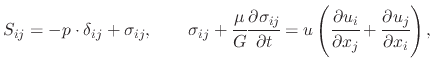   $$S_{ij}=-p\cdot\delta_{ij}+\sigma_{ij},\qquad\sigma_{ij}+\cfrac{\m... ...{\partial u_{i}}{\partial x_{j}}+\cfrac{\partial u_{j}}{\partial x_{i}}\right),$$ (85)

   
   
   where $u_i$ is a velocity component.

   The system of equations (3.13) and (3.14) make up the Stoke's equations with the boundary conditions

   $$\vec{u}\vert _{Si\slash SiO_{2}}=\cfrac{\gamma-1}{\gamma}\cdot\cf... ...ad \left[p\right]-\left[\mu\cdot n_{i}\sigma_{ij}n_{j}\right]=\beta\cdot\kappa,$$ (86)

   
   
   where $\left[\cdot\right]$ denotes the jump across a liquid-liquid interface, $\beta$ is the surface tension coefficient, and $\kappa$ is the surface curvature.

4. Propagation of the interfaces in the deformation velocity field is the step during which all interfaces above the Si-SiO$_2$ interface are updated. This includes the SiO$_2$-Nitride interface, SiO$_2$-ambient interface, and Nitride-ambient interface. The interfaces are updated using the LS representation

   $$\cfrac{\partial\Phi}{\partial t}+\vec{u}\cdot\vec{\nabla}\phi.$$ (87)

   
   

The main advantage of the LS method when compared to the FEM for solving visco-elastic problems is that all potential errors which arise due to unstructured mesh irregularities are removed. The LS also makes it very easy to follow shape topologies which change with time. The LS method natively handles complex surfaces, which can split or recombine during a simulation process.