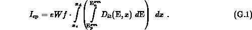
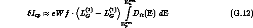
The expression will be derived for method II discussed in the main text. In this method the trapezoidal pulses with all parameters fixed are applied on the gate, while the drain-bulk reverse bias is changed. Drain and source are connected together. Let us assume that:
 and the drain side
  depend on the reverse
bias
depend on the reverse
bias  ,
,
 and
and
 ,
,
 .
.
The capture cross-sections occurring as  and
and
 in the expressions for the emission levels are
assumed to be spatially constant. Differentiating G.1 with
respect to the reverse bias
in the expressions for the emission levels are
assumed to be spatially constant. Differentiating G.1 with
respect to the reverse bias  it follows without any simplification
The factors  can be approximated as follows:
From the relationship between the emission times and the emission levels, 3.66 and 3.81, one obtains
Differentiating the expressions for the emission times in the trapezoidal wave-form charge-pumping technique (3.77) it follows
where  and
and  are the charge-pumping threshold and
flat-band voltage which determine the start and the end of the
non-steady-state electron emission.
are the charge-pumping threshold and
flat-band voltage which determine the start and the end of the
non-steady-state electron emission.  and
and  are the
corresponding levels for the non-steady-state hole emission.
It may be adopted that
are the
corresponding levels for the non-steady-state hole emission.
It may be adopted that  and
and  are nearly equal to each other when
  and
and  are comparable, finally
resulting in
are comparable, finally
resulting in
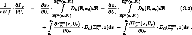
Employing G.6, relationship G.2 can be simplified. In the following, special cases are discussed.
Symmetrical case (virgin devices):
We assume that
holds. After replacing G.7 in G.2, with benefit of G.6, it follows
Several aspects deserve attention here:
Note that the active interval in the energy gap
 changes explicitly with
and also because both,
changes explicitly with
and also because both,  and
and  change
explicitly with the
change
explicitly with the  -coordinate as well. Therefore, the active
energy interval in the band gap is not constant in this lateral
profiling technique, but changes during the course of experiment. This
is not very convenient, particularly when both and (or
) are varied in order to scan .
-coordinate as well. Therefore, the active
energy interval in the band gap is not constant in this lateral
profiling technique, but changes during the course of experiment. This
is not very convenient, particularly when both and (or
) are varied in order to scan .
 represents the experimental result.
This factor is positive.
, the potential
decreases (in the junctions), increases,
represents the experimental result.
This factor is positive.
, the potential
decreases (in the junctions), increases,
 increases and consequently,
 , this term is negative.
 is a positive factor which can be obtained
by numerical steady-state calculation.
is a positive factor which can be obtained
by numerical steady-state calculation.
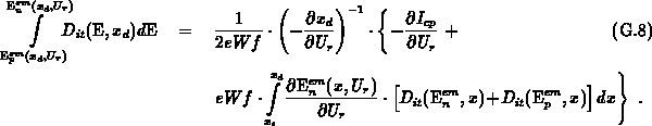
For the purpose of model-evaluation, the parasitic term which contains
 can be calculated in different ways.
Since the dominant contribution to this factor comes from the channel region and
less from the junctions, we can evaluate this term in the channel region and
apply it for the interface in complete. In order to calculate this factor we
further assume that the traps are uniformly distributed in the channel (they
can vary in the junctions). Approaches we analyzed are listed:
can be calculated in different ways.
Since the dominant contribution to this factor comes from the channel region and
less from the junctions, we can evaluate this term in the channel region and
apply it for the interface in complete. In order to calculate this factor we
further assume that the traps are uniformly distributed in the channel (they
can vary in the junctions). Approaches we analyzed are listed:
 located in the middle of the channel. In G.2,
only the parasitic term remains
located in the middle of the channel. In G.2,
only the parasitic term remains
The term  results from numerical
simulation. In a first approximation, the factor
results from numerical
simulation. In a first approximation, the factor
 may be assumed as
constant along the whole interface.
may be assumed as
constant along the whole interface.
 versus and approximating
 . Further, we benefit from
valid in the channel only.  follows
by numerical differentiation of the calculated
follows
by numerical differentiation of the calculated  .
.
 and
and  . The difference in measured currents
becomes
. The difference in measured currents
becomes
for traps uniformly distributed in the channel region. The second
parasitic term in G.8 follows after numerical
differentiation  .
.
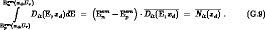
 distributions. Experimental work is necessary here. Nevertheless, using
all the methods noted above we have evaluated the parasitic term and
have shown that expression G.8 provides correct results.
Therefore, no additional undesired effects occur in this kind of charge-pumping
experiment.
distributions. Experimental work is necessary here. Nevertheless, using
all the methods noted above we have evaluated the parasitic term and
have shown that expression G.8 provides correct results.
Therefore, no additional undesired effects occur in this kind of charge-pumping
experiment.
Note that in the investigation in Section 3.5.2 we
calculate an average trap density in the energy space  instead
of the total density
instead
of the total density  actually scanned. The active energy interval
 has also been obtained by the methods
discussed above.
has also been obtained by the methods
discussed above.
Non-symmetrical case (stressed device):
The interface trap density in the stressed device can be represented by
 , where
  is the trap density in the virgin device. The stress-generated traps
  are localized near the drain junction
 . We assume that the boundary after the stress at the source
side is the same as before stress
. We assume that the boundary after the stress at the source
side is the same as before stress  . If we assume that the
stress-generated traps do not influence the capture boundary at the drain side
. If we assume that the
stress-generated traps do not influence the capture boundary at the drain side
 , it follows
where  is the charge-pumping current in the virgin device. The second
parasitic term is small for the strongly localized traps in comparison with the
desired factor due to scanning of the interface. This term may be omitted in
practice. The main contribution to this factor is from the channel region and
it vanishes when processing the differential
is the charge-pumping current in the virgin device. The second
parasitic term is small for the strongly localized traps in comparison with the
desired factor due to scanning of the interface. This term may be omitted in
practice. The main contribution to this factor is from the channel region and
it vanishes when processing the differential  characteristics
instead of
characteristics
instead of  . A general expression which accounts for the influence of
the stress-generated traps on the capture boundary (
. A general expression which accounts for the influence of
the stress-generated traps on the capture boundary ( ) can be
trivially derived. It is omitted here.
) can be
trivially derived. It is omitted here.
Constant amplitude technique:
In this method all parameters of the trapezoidal gate pulse are constant. The
top level is sufficiently high so that the complete interface is inverted during
the course of experiment. The reverse bias is kept constant. The interface
is scanned by changing the gate bottom level  . The emission times do
not change with , but only the active interface area changes.
Differentiating G.1 with respect to it follows
. The emission times do
not change with , but only the active interface area changes.
Differentiating G.1 with respect to it follows
In symmetrical cases  may be assumed.
With benefit of G.7 it follows
may be assumed.
With benefit of G.7 it follows