 and electrons
When compared to n-type semiconductors, some of the equations from (B.1) to
(B.13) differ for p-type semiconductors. Due to their exchanged concentrations of
holes and electrons
![1 qp [ (n ) ]
-E2s = --p0- (exp(− βψs)+ β ψs − 1) + --p0 (exp (β ψs)− βψs − 1)
2 ϵrϵ0β pp0](diss2102x.png) |
 | (B.14) |
with
 | (B.15) |
the space-charge-density becomes
 | (B.16) |
Again, the charge at the surface (B.16) can be approximated for certain
surface potentials  .
.
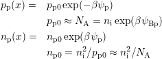
For accumulation with  , the term
  dominates the root in
(B.15), making
dominates the root in
(B.15), making 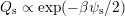 .
.
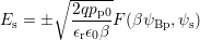
Starting from the flatband condition at  , first depletion of holes and
afterwards weak inversion set in till
, first depletion of holes and
afterwards weak inversion set in till  is fulfilled. In these two regimes
 .
.
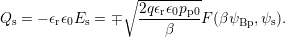
Finally, beyond  the first term in (B.15), starts to dominate
by outbalancing the negative exponent in
the first term in (B.15), starts to dominate
by outbalancing the negative exponent in  which yields
 .
.
In Fig. B.2 the different operating conditions with its resulting surface charge
density  at the interface side of the semiconductor are opposite for both
p-type and n-type semiconductors. The above mentioned approximations very
well fit the exact solutions (B.13) and (B.16), as deviations are only present at
the intersections of the different regimes. Furthermore, it is shown that
at the interface side of the semiconductor are opposite for both
p-type and n-type semiconductors. The above mentioned approximations very
well fit the exact solutions (B.13) and (B.16), as deviations are only present at
the intersections of the different regimes. Furthermore, it is shown that
 , where the subscripts
  and
and  denote the type of
semiconductor.
denote the type of
semiconductor.