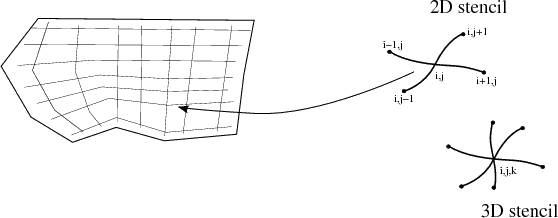
The finite difference discretization scheme is one of the simplest forms of discretization and does not easily include the topological nature of equations. A classical finite difference approach approximates the differential operators constituting the field equation locally. Therefore a structured grid is required to store local field quantities. For each of the points of the structured grid the differential operators appearing in the main problem specification are rendered in a discrete expression. The order of the differential operator of the original problem formulation directly dictates the number of nodes to be involved.
Here, the main drawback of finite differences can already be seen. The association of physical field values only to points cannot handle higher dimensional geometrical objects. Furthermore, the n-point discretization given by the order of the original formulation only includes the logically direct orthogonal neighbors while the other neighbors are neglected, depicted in Figure 2.8.
The advantages of this method are that it is easy to understand and to implement, at least for simple material relations. The finite difference method optimizes the approximation for the differential operator in the central node of the considered patch. Enhancements related to the use of non-orthogonal grids and the low order of accuracy were developed but have not proven successful.
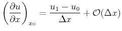
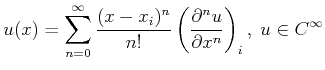
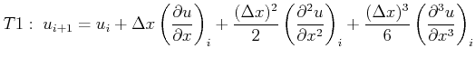
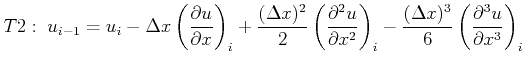
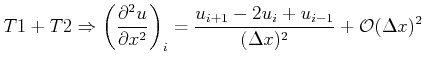
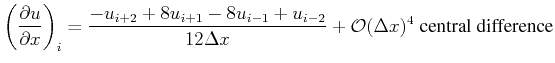
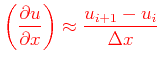
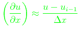
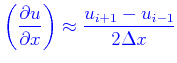
The derivatives of the partial differential equation are approximated by linear combinations of function values at the structured grid points. Arbitrary order approximations can be derived from a Taylor series expansion:
 |
(2.47) |
A geometric interpretation of the different equations is shown in Figure 2.9.
|
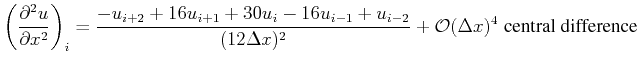
For second-order derivatives the central difference scheme can be used:
 |
(2.48) |
 |
(2.49) |
 |
(2.50) |
The accuracy of the finite difference approximations is given by:
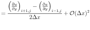
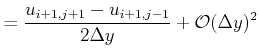
Mixed derivatives, illustrated in Figure 2.10 can be approximated, e.g., for two dimensions by:
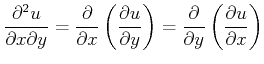 |
(2.51) |
A second-order finite difference approximation for two dimensions results in:
 |
(2.52) |
Boundaries also have to be handled by the finite difference method, see Figure 2.11,
|
but at the boundary on the left side, the backward and central
difference approximations would need ![]() which is not
available. Therefore treatment of boundaries is more complex for the
finite difference method compared to the other discretization
schemes. This particular problem grows in complexity if higher order
discretization schemes are used, because more grid points are required
to evaluate the corresponding approximation.
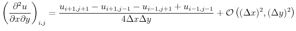
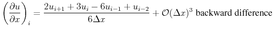
Higher order approximations with finite differences are given by, e.g.:
which is not
available. Therefore treatment of boundaries is more complex for the
finite difference method compared to the other discretization
schemes. This particular problem grows in complexity if higher order
discretization schemes are used, because more grid points are required
to evaluate the corresponding approximation.
Higher order approximations with finite differences are given by, e.g.:
 |
(2.54) |
 |
(2.55) |
 |
(2.56) |
 |
(2.57) |
One method of directly transfering the discretization concepts (Section 2.1) is the finite difference time domain method. It is analyzed here related to time-dependent Maxwell equations, as was first introduced by Yee [30]. It is one of the exceptional examples of engineering illustrating great insights into discretization processes.
With this method, the partial spatial and time derivatives are replaced by a finite difference approximation. This system is solved using an explicit time evaluation. One of the main advantages of this method is that no matrix operations or algebraic solution methods have to be used.
The spatial domain is discretized by two dual orthogonal regular
Cartesian grids based on cubes with spatial subdivisions of
![]() , whereas the time domain is subdivided into
intervals of
, whereas the time domain is subdivided into
intervals of ![]() . The original formulation was based on
half-step staggered grids in space and time. The quantities from the
second complex are denoted with
. The original formulation was based on
half-step staggered grids in space and time. The quantities from the
second complex are denoted with
![]() . It is important to highlight that two
different grids are necessary, due to the fact that different
quantities with different orientation reside on these two distinct
grids, even if in this method the secondary quantities coincide
numerically with the primary ones.
. It is important to highlight that two
different grids are necessary, due to the fact that different
quantities with different orientation reside on these two distinct
grids, even if in this method the secondary quantities coincide
numerically with the primary ones.
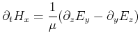
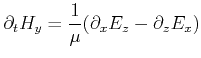
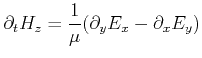
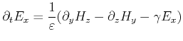
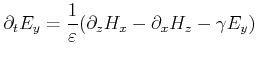
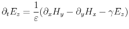
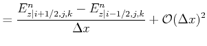
Maxwell's equations, given in Section 1.2, if projected onto a regular Cartesian structured grid, yield the following six coupled scalar equations:
 |
(2.58) |
 |
(2.59) |
 |
(2.60) |
 |
(2.61) |
 |
(2.62) |
 |
(2.63) |
These equations are the basic expressions for the finite difference time domain method (FDTD). The divergence relations are fulfilled by this method implicitly.
The components of the electric and magnetic field
![]() and
and
![]() with their corresponding projections to the coordinate
axes are the variables used. These variables and the local values of
material properties are attached to the midpoints of the grid
edges. The variable indexing scheme is also used consistently with
[30]
with their corresponding projections to the coordinate
axes are the variables used. These variables and the local values of
material properties are attached to the midpoints of the grid
edges. The variable indexing scheme is also used consistently with
[30]
| (2.64) |
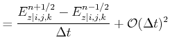
With this notation the following expressions are obtained with central difference approximation:
 |
(2.65) | |
 |
(2.66) |
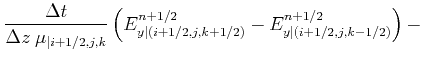
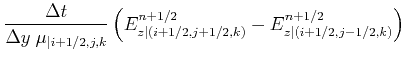
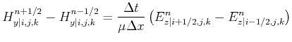
The time-stepping formulas for ![]() are:
are:
| (2.67) | ||
 |
||
 |
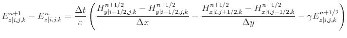
and the time-stepping for ![]() :
:
| (2.68) | ||
 |
||
 |
As already introduced, the FDTD method does not use global
quantities. Instead only local nodal values of the corresponding
vector values are used. Based on the initial problem formulation, it
can be seen that these local values are the projections of averaged
field components onto 2-cells, and therefore are local representatives
of the global quantities. With local constitutive relations (only the
![]() part is given):
part is given):
| (2.69) |
| (2.70) |
| (2.71) | ||
| (2.72) | ||
| (2.73) |
| (2.74) | ||
| (2.75) |
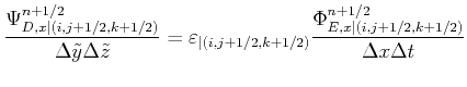
Rewriting Equation 2.72 and Equation 2.76 yields:
 |
(2.76) | |
 |
(2.77) |
which can be expressed for ![]() and
and ![]() . For
. For ![]() it reads:
it reads:
 |
(2.78) |
while the result for ![]() is:
is:
 |
(2.79) |
Therefore this equation represents a discrete constitutive equation of
the simplest type, obtained by extending the local constitutive
equations
![]() , and
, and
![]() with the assumption of planarity, regularity, and
orthogonality of the cells.
with the assumption of planarity, regularity, and
orthogonality of the cells.
Examining the time-stepping formulae for ![]() , the time-stepping for
, the time-stepping for
![]() becomes:
becomes:
| (2.80) | ||
and from the ![]() and the corresponding
and the corresponding
![]() is obtained:
is obtained:
| (2.81) | ||
The expressions can then be transformed into equations depending only on two global values:
For the special case of a dominant magnetic system, TM-mode, the following expressions can be derived:
 |
(2.83) | |
 |
(2.84) | |
 |
(2.85) |
With these expressions the TM-mode at
![]() is discretized by:
is discretized by:
|
(2.86) | |
|
(2.87) |
 |
(2.88) |
 |
(2.89) |
For a dominant electric system, the TE-mode is given by:
|
(2.90) |
|
(2.91) |
|
(2.92) |
With these expressions the TE-mode at
![]() is
discretized by:
is
discretized by:
|
(2.93) |
 |
(2.94) |
As can be seen, the ![]() values for the full time-steps and the
values for the full time-steps and the
![]() ,
, ![]() for half time-steps are already available, and the the
update for
for half time-steps are already available, and the the
update for ![]() ,
, ![]() can be done without any further
calculation. On the contrary
can be done without any further
calculation. On the contrary
![]() is not available
and has to be approximated by:
is not available
and has to be approximated by:
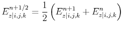 |
(2.95) |
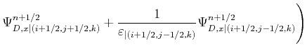
From this the following expression is finally obtained:
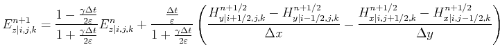 |
(2.96) |
As can be seen only the neighboring values ![]() ,
, ![]() are used to
evaluate the spatial derivative of
are used to
evaluate the spatial derivative of ![]() . Also, only the neighboring
elements of
. Also, only the neighboring
elements of ![]() ,
, ![]() and
and ![]() are used to calculate the spatial
derivatives of
are used to calculate the spatial
derivatives of ![]() ,
, ![]() . Therefore this method calculates both
fields,
. Therefore this method calculates both
fields,
![]() and
and
![]() , based on the
, based on the
![]() expressions
with special requirements on the given field. Note this
discretization can also be derived by the global integral
discretization [33], which eases the evaluation
of boundary conditions.
expressions
with special requirements on the given field. Note this
discretization can also be derived by the global integral
discretization [33], which eases the evaluation
of boundary conditions.
![\begin{figure}\begin{center}
\small
\psfrag{u} [c]{$u(x)$}
\psfrag{dx} [c]{...
...discretization_fd_geometric.eps, width=0.9\textwidth}
\end{center}
\end{figure}](img543.png)
![\begin{figure}\begin{center}
\small
\psfrag{yi+1} [c]{$y_{j+1}$}
\psfrag{yi...
...res/discretization_fd_mixedderivative.eps, width=9cm}
\end{center}
\end{figure}](img553.png)


![\begin{figure}\begin{center}
\small\psfrag{x-1} [c]{$x_{-1}$}\psfrag{x0} [c]...
...discretization_fd_boundaries.eps, width=0.4\textwidth}\end{center}\end{figure}](img561.png)