The finite element method is a systematic approach to approximate the
unknown exact solution of a partial differential equation based on
basis functions and the projection of a given domain onto a consistent
finite cell complex. The finite elements correspond to the ![]() -cells
of the complex.
-cells
of the complex.
The origin of the finite element method is in the solid mechanics of rigid bodies [29]. Some constraints should be placed on the selection of the shape functions to guarantee the fact that with an arbitrary number of shape functions the exact solution is approximated best, and in the limit, the exact solution should be obtained.
A good approximation is obtained by a residual formulation where the residuum is formulated as the difference of the unknown exact solution and the calculated approximate solution. This residuum is weighted over the simulation domain and integrated with the requirement that the integral vanishes with a set of linearly independent weighting functions. The other possible mechanism is the variational formulation of the partial differential equation [28,68].
One of the main advantages of the finite element method is the possibility to adapt the basis functions to the eigenfunctions of the differential operators [28]. Thereby a high precision of this method can be obtained with a moderate number of mesh elements. Different areas of materials as well as anisotropic, inhomogeneous, and non-linear quantities can be treated. If no boundary conditions are declared, homogeneous/natural Neumann boundary conditions are implicitly given.
In the following, a theoretical part of the finite element method is
summarized, which is a special Galerkin method
[28,29] based on the following
construction of finite dimensional subspaces
![]() :
:
which is defined on an arbitrary dimensional, single connected domain
![]() with boundary
with boundary
![]() . Equation
2.22 is fulfilled by
functions of class
. Equation
2.22 is fulfilled by
functions of class ![]()
| (2.23) |
The notation
![]() being a linear spatial differential
operator.
Additionally, it is assumed that the domain
being a linear spatial differential
operator.
Additionally, it is assumed that the domain
![]() has a piecewise
smooth boundary
has a piecewise
smooth boundary
![]() . A general form of boundary conditions can thereby be specified by:
. A general form of boundary conditions can thereby be specified by:
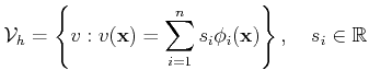
The infinite-dimensional space
![]() is then replaced by a
sequence of finite-dimensional spaces
is then replaced by a
sequence of finite-dimensional spaces
![]() with
with ![]() linearly
independent functions
linearly
independent functions
![]() which span the space
which span the space
![]() , e.g.,
, e.g.,
 |
(2.26) |
| (2.27) |
By selecting
![]() the following system is obtained:
the following system is obtained:
The solution variable ![]() is then also expanded in terms of the basis
is then also expanded in terms of the basis
![]() of
of
![]() .
.
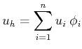 |
(2.29) |
A graphical representation of ![]() is given in Figure
2.7.
is given in Figure
2.7.
![\begin{figure}\begin{center}
\small\psfrag{f} [c]{$\mathrm{u}$}\psfrag{x} [c...
...e=figures/fe_ansatz_function.eps, width=0.5\textwidth}\end{center}\end{figure}](img513.png) |
By the given selection of the test function and the expansion of the
solution variable, it can be observed [69] that the
scalar product in Equation 2.28 transforms
the differential operator
![]() into the discrete operator
into the discrete operator
The residuum is obtained by using the operator of Equation 2.30
| (2.31) |
The next step for the discrete approximation of a given problem is the
subdivision of the domain
![]() according to cell complex
properties (see Section
1.3 for details). The elements of the
cell complex, the collection of cells, is then used as finite elements
for the finite space
according to cell complex
properties (see Section
1.3 for details). The elements of the
cell complex, the collection of cells, is then used as finite elements
for the finite space
![]() . The basis functions
. The basis functions
![]() are defined on the global vertices
are defined on the global vertices
![]() ,
the 0-cells, only and are therefore called nodal basis functions. They
can be expressed as:
,
the 0-cells, only and are therefore called nodal basis functions. They
can be expressed as:
| (2.32) |
Based on this subdivision of the finite element space, the function
![]() can be expressed in local cell terms by
can be expressed in local cell terms by
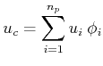 |
(2.33) |
| (2.34) |
and the local residuum is then defined as:
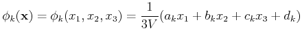
To determine the operator given in Equation 2.35 for a particular cell type, the basic nodal functions have to be calculated, e.g., for a 3-simplex cell (tetrahedron):
 |
(2.36) |
The key for an efficient practical realization is that global finite
elements are defined as transformations of a reference element in a
normalized coordinate system. Each point of the cell
![]() can be expressed as a bijective function onto a
reference point
can be expressed as a bijective function onto a
reference point
![]() :
:
| (2.41) | |
| (2.42) | |
| (2.43) | |
| (2.44) |
Equation 2.37 is then calculated by:
 |
(2.45) |
where
![]() is the Jacobian of the projection Equation 2.38 - Equation 2.40.
The final assembly process consists of calculating stencil matrices
is the Jacobian of the projection Equation 2.38 - Equation 2.40.
The final assembly process consists of calculating stencil matrices
![]() for each element of the cell complex, mapping the
local vertex indices to a global index and then building the global
matrix
for each element of the cell complex, mapping the
local vertex indices to a global index and then building the global
matrix
![]() .
.
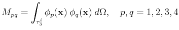
For an electrostatic problem formulated by the Laplace equation
![]() the stencil matrix is represented by:
the stencil matrix is represented by:
 |
(2.46) |