


 Previous: 3.3.5.2 Follow-Each-Recoil Method
Up: 3.3.5 Material Damage -
Next: 3.3.5.4 Amorphization
Previous: 3.3.5.2 Follow-Each-Recoil Method
Up: 3.3.5 Material Damage -
Next: 3.3.5.4 Amorphization
3.3.5.3 Point Defect Recombination
Besides the energy loss mechanism of mobile particles and the damage generation
process, thermal effects have to be considered when simulating ion
implantation. All atoms in a solid perform random
motions which result in diffusion effects of impurities and point
defects. Thereby interstitials and vacancies can approach each other close enough to
recombine to a regular lattice atom.
Several approaches have been proposed to model this recombination effect either in
combination with the Kinchin-Pease damage model or in combination with the
Follow-Each-Recoil method.
An empirical model which can be combined with the Kinchin-Pease model is
given in [75]. The recombination process is subdivided into
recombination within a single cascade and recombination with point defects from
previous cascades. The number of point defects surviving recombination within a
single cascade is determined by an ion species dependent factor
 (recombination factor) which is multiplied with the number of
generated point defect pairs
(recombination factor) which is multiplied with the number of
generated point defect pairs  calculated by the modified Kinchin-Pease model
(3.143). The recombination with previously generated point
defects is considered by a recombination probability
calculated by the modified Kinchin-Pease model
(3.143). The recombination with previously generated point
defects is considered by a recombination probability  . The expected
value of Frenkel pairs
. The expected
value of Frenkel pairs
 remaining after recombination per
generated Frenkel pair can be calculated by
remaining after recombination per
generated Frenkel pair can be calculated by
 |
(3.149) |
The first term takes into account that the vacancy and the interstitial do not
recombine which results in an additional Frenkel pair. The probability of this
process is
 . The second terms considers a full recombination process
with a probability of
. The second terms considers a full recombination process
with a probability of  , which reduces the number of Frenkel pairs by
one.
, which reduces the number of Frenkel pairs by
one.
is assumed to be proportional to the local interstitial and vacancy
concentration  ,
,  and to a species dependent saturation concentration
 .
.
 |
(3.150) |
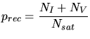
Combining all contributions the total number of new stable point defects
 generated by a primary recoil can therefore be calculated by
 |
(3.151) |
This expression is more general than the one proposed in [75] where the
vacancy and interstitial concentration are assumed to be
equal. Tab. 3.5 summarizes experimentally determined values
of and ([7], [73], [74],
[75]). A similar model was proposed by Posselt in [63]. The
models mainly differ in placing the interstitials as will be explained in
Sec. 3.3.5.
Table 3.5:
Parameters for the empirical recombination model for different ion species.
| Ion species |
|
|
| Boron |
0.125 |
 cm cm |
| Phosphorus |
1.000 |
 cm cm |
| Arsenic |
2.000 |
 cm cm |
|
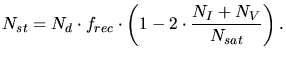
There are several approaches to model the point defect recombination process if
a Follow-Each-Recoil method is applied for the calculation of the point defects
([32], [46], [85], [86]). All these
methods are based in principle on the same concepts which will be summarized in
the following by looking in detail at the damage generation processes.
- When a mobile particle transfers more energy than the displacement energy to a
stable atom in a crystalline solid a recoil is generated. If this recoil is
removed from a lattice position a vacancy is left behind. If an interstitial
atom was hit the number of interstitials is reduced by one.
 |
(3.152) |
 |
(3.153) |
and are the number of interstitials and vacancies,
 and
indicate the change in the number of interstitials and
vacancies, respectively.
and
indicate the change in the number of interstitials and
vacancies, respectively.
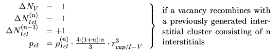
- If a vacancy has been generated it can recombine with an
interstitial.
 |
(3.154) |
 |
(3.155) |
There are two approaches to model the recombination probability . By
the first approach ([46]) it is assumed that the recombination
probability is a linear function of the interstitial concentration  .
.
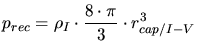 |
(3.156) |
 is a capturing radius for interstitial-vacancy pairs.
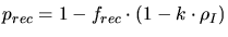
By the alternative approach ([32]) it is also suggested to
distinguish between the recombination of point defects originating from the same
cascade and point defects originating from different cascades. While the
recombination of point defects originating from different cascades is assumed to
be linearly proportional to the interstitial concentration, the recombination
of point defects originating from the same cascade is assumed to be constant
(independent of the interstitial concentration). In order quantify this assumption
a constant value  is added for the calculation of the
recombination probability.
is added for the calculation of the
recombination probability.
 |
(3.157) |
is the recombination probability within a single cascade and
 is the proportionality coefficient for inter-cascade recombination.
- Instead of recombining with an interstitial a vacancy can recombine with
an impurity atom which is located at an interstitial site.
 |
(3.158) |
 |
(3.159) |
|
(3.160) |
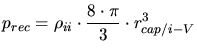 |
(3.161) |
 is a capturing radius for impurity-vacancy pairs. A different
capturing radius is required for each impurity species because their thermal
mobilities are different.
is a capturing radius for impurity-vacancy pairs. A different
capturing radius is required for each impurity species because their thermal
mobilities are different.  is the number of activated (located at
lattice positions) impurities,
is the number of activated (located at
lattice positions) impurities,  and
and  are the number and the
concentration of interstitial impurities.
are the number and the
concentration of interstitial impurities.
- When a mobile particle comes to rest an interstitial atom is generated.
![$\displaystyle \Delta N_I = +1 \;\;\;\; \mathrm{\text{\parbox[t]{0.4\textwidth}{if the particle is an atom of the target material}}}$](img451.gif) |
(3.162) |
![$\displaystyle \Delta N_{ii} = +1 \;\;\;\; \mathrm{\text{\parbox[t]{0.4\textwidth}{if the particle is an impurity}}}$](img452.gif) |
(3.163) |
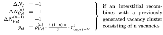
- Such an interstitial atom can recombine with a previously generated
vacancy.
![$\displaystyle \left. \begin{array}{rl} \Delta N_I &= -1\\ \Delta N_V &= -1\\ ...
...\parbox[c]{0.35\textwidth}{if the particle is an atom of the target material}}}$](img453.gif) |
(3.164) |
![$\displaystyle \left. \begin{array}{rl} \Delta N_{ii} &= -1\\ \Delta N_{ai} &= ...
...\;\; \mathrm{\text{\parbox[t]{0.35\textwidth}{if the particle is an impurity}}}$](img454.gif) |
(3.165) |
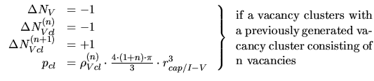
- Besides recombination the point defects can form clusters as indicated by
several molecular dynamic simulations ([15], [65]) and
isolated point defects can recombine with these clusters. The reaction radius of
a cluster which determines the clustering probability
 is assumed to be
![$ r_{cap/cl} = \sqrt[3]{n}\cdot r_{cap/{I-V}}$](img456.gif) ([85]).
([85]).
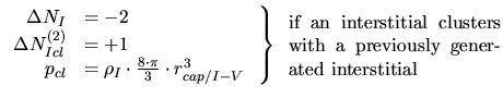 |
(3.166) |
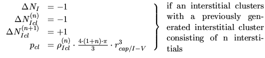 |
(3.167) |
![$\displaystyle \left. \begin{array}{rl} \Delta N_V &= -2\\ \Delta N_{Vcl}^{(2)}...
...c]{0.35\textwidth}{if a vacancy clusters with a previously generated vacancy}}}$](img459.gif) |
(3.168) |
 |
(3.169) |
 |
(3.170) |
 |
(3.171) |
 ,
,
 ,
,
 ,
,
 are the
densities and numbers of interstitial and vacancy clusters consisting of
are the
densities and numbers of interstitial and vacancy clusters consisting of  point defects.
Applying these mechanisms the generation of several defect species
like isolated interstitials and vacancies, impurity-interstitial pairs and point
defect and impurity-point defect clusters can be modeled. But at least isolated
interstitials and vacancies have to be considered in the simulation to
correctly handle the de-channelling mechanism. Therefore at least the mechanisms
mentioned in 1., 2. and 4. have to be applied during the simulation, while all
other mechanisms just provide additional information for the output of the
Monte-Carlo ion implantation simulation.
Previous: 3.3.5.2 Follow-Each-Recoil Method
Up: 3.3.5 Material Damage -
Next: 3.3.5.4 Amorphization
A. Hoessiger: Simulation of Ion Implantation for ULSI Technology