Subsections

• 3.2.1 Oxidant Diffusion
• 3.2.2 Dynamics of ${\eta }$
• 3.2.3 Volume Expansion of the New Oxide
• 3.2.4 Diffusion Coefficient and Reaction Layer
• 3.2.5 Mechanics
  • 3.2.5.1 Elastic Mechanical Model
  • 3.2.5.2 Visco-Elastic Mechanical Model
  • 3.2.5.3 Volume Increase and Mechanics

3.2 Mathematical Formulation

From the mathematical point of view the whole oxidation process can be described by a coupled system of partial differential equations, one for the diffusion of oxidants through SiO$_2$, the second for the conversion of Si into SiO$_2$ at the interface, and a third for the mechanical problem of the complete oxidized structure.

3.2.1 Oxidant Diffusion

The diffusion of oxidants in the domains $\Omega_1$, $\Omega_2$, and $\Omega_3$ according to Fig. 3.1 is described by

$$D(T) \Delta C(\vec{x},t) = k(\eta) C(\vec{x},t),$$ (3.2)

where $\Delta = \frac{\partial^2}{\partial x^2}+ \frac{\partial^2}{\partial y^2}+ \frac{\partial^2 }{\partial z^2}$ is the Laplace operator, $C(\vec{x},t)$ is the oxidant concentration in the material, and $D(T)$ is the temperature dependent low stress diffusion coefficient.
The boundary conditions for the diffusion equation (3.2) are

$$C=C^* \quad \mathrm{on} \quad \Gamma_1 \qquad \mathrm{and} \qquad... ...partial C}{\partial n} =0 \quad \mathrm{on} \quad \Gamma_2, \Gamma_3, \Gamma_4,$$ (3.3)

where $C^*$ is the oxidant concentration in the gas atmosphere. $\frac{\partial C}{\partial n} =0$ is a Neumann boundary condition, which means that there does not exist an oxidant flow through these boundaries.
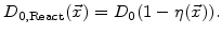
In (3.2) $k(\eta)$ is the strength of a spatial sink and not just a reaction coefficient at a sharp interface [67]. $k(\eta) C(\vec{x},t)$ defines how many particles of oxygen per unit volume are transformed in a unit time interval to oxide. $k(\eta)$ is defined to be linearly proportional to $\eta(\vec{x},t)$

$$k(\eta)= \eta(\vec{x},t) k_{{max}},$$ (3.4)

where $k_{max}$ is the maximal possible strength of the sink.

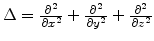
Figure 3.1: Schematic domains and boundaries.

3.2.2 Dynamics of $\boldsymbol{\eta}$

Because of the chemical reaction which consumes silicon, the normalized silicon concentration $\eta$ is changed. In a test volume $\Delta V$, where is assumed that the oxidant concentration C is constant during a time interval $\Delta$$t$ there are $k(\eta) C(\vec{x},t) \Delta V \Delta t$ particles of oxygen which react with $k(\eta) C(\vec{x},t) \Delta V \Delta t/(\lambda N_1)$ unit volumes of silicon. By this process the silicon concentration is reduced.
The dynamics of $\eta$ can be described by [67]

$$\frac{\partial \eta(\vec{x},t)} {\partial t} = - \frac{1}{\lambda} k(\eta) C(\vec{x},t)/N_1,$$ (3.5)

where $\lambda$ is the volume expansion factor (=2.25) for the reaction from Si to SiO$_2$, and $N_1$ is the number of oxidant molecules incorporated into one unit volume of SiO$_2$.

In this model the dynamics of $\eta$ is equivalent with the movement of the sharp Si/SiO$_2$ interface in the standard model, because $\eta$ defines the silicon and oxide areas. The only difference is that here a diffuse interface (Fig. 3.1) moves, where is a mixture of silicon and oxide.

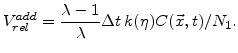
3.2.3 Volume Expansion of the New Oxide

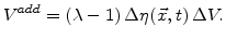
Because of the much lower density of oxide compared with silicon, the conversion from Si to SiO$_2$ leads to a significant volume increase of the new oxide. In the advanced model the conversion is not performed instantaneously, it needs some finite time. The fraction of SiO$_2$ in a small volume $\Delta V$ is expressed by the $\eta$ value. The new generated oxide in the reaction layer is described by the change of $\eta$. For a time period $\Delta t$ the $\eta$-value and the silicon fraction decreases with

$$\Delta \eta(\vec{x},t) = - \frac{1}{\lambda} \Delta t k(\eta) C(\vec{x},t)/N_1.$$ (3.6)

The additional volume in a test volume $\Delta V$ is given by

$$V^{add}= (\lambda-1) \Delta \eta(\vec{x},t) \Delta V.$$ (3.7)

Because the maximal volume increase of the oxide is limited to 1.25 times of the volume of original silicon, $V^{add}$ in (3.7) must be scaled with ($\lambda-1$).

The normalized additional volume with (3.6) and (3.7) after a time $\Delta t$ is

$$V^{add}_{rel} = \frac{\lambda - 1}{\lambda}\Delta t k(\eta) C(\vec{x},t)/N_1.$$ (3.8)

An important aspect of (3.8) is that the sum of $V^{add}_{rel}$ over all time steps can not be more than 125%, which is the maximal volume increase of the material during oxidation.

3.2.4 Diffusion Coefficient and Reaction Layer

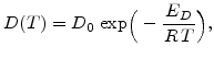
In contrast to the standard models, where the diffusion coefficient $D(T)$ is automatically included in the parabolic rate constant B, in the advanced model $D(T)$ must be determined separately for the specific temperature and oxidant species. The most interesting oxidant species come from dry and wet oxidation.

In general the diffusion coefficient follows the expression

$$D(T)=D_0\;\mathrm{exp}\Big(-\frac{{E_D}}{{R T}}\Big), \vspace*{-1mm}$$ (3.9)

where $D_0$ is a pre-exponential diffusion constant, $E_D$ is the activation energy in [cal], T the temperature in [K], and $R$ is the universal gas constant with $R=1.987$ cal/(K$\cdot$mol).

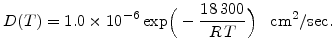
For dry oxygen ambients the results of Norton [68] can be used, who found that the activation energy for diffusion of oxygen in vitreous silica is 27 kcal and the diffusion coefficient $D(T)$ is 4.2 $\times 10^{-9}$ cm$^2$/sec (= 0.42 $\mu$m$^2$/sec) at a temperature of 950$^{\circ }$C. With these data it is possible to calculate $D_0$, and (3.9) can be written for dry oxidation in the form

$$D(T)=2.82\times 10^{-4} \mathrm{exp}\Big(-\frac{27 000}{R T}\Big)\;\;\;\mathrm{cm^2/sec}. \vspace*{-1mm}$$ (3.10)

For wet oxidation the results from Moulson and Roberts [69] are most suitable. They have investigated heated silica glass in water vapour between 600 and 1200$^{\circ }$C and found the temperature dependent diffusion coefficient

$$D(T)=1.0\times 10^{-6} \mathrm{exp}\Big(-\frac{18 300}{R T}\Big)\;\;\;\mathrm{cm^2/sec}. \vspace*{-1mm}$$ (3.11)

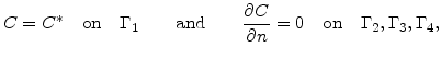
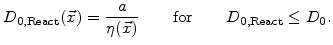
In the advanced model the reaction layer has a spatial finite width d $_{\mathrm{React}}$, which can vary. This width is mainly determined by the value of $k_{max}$. The bigger $k_{max}$, the steeper the concentration decay and the thinner the reaction layer. Therefore, d $_{\mathrm{React}}$ is inverse proportional to $k_{max}$ and so the width can be controlled by $k_{\mathrm{max}}$. This means that a small value of $k_{max}$ (e.g. $k_{\mathrm{max}} \approx 50$) leads to a wide reaction layer (e.g d $_{\mathrm{React}} \approx 100$ nm) and a big value of $k_{max}$ (e.g. $k_{\mathrm{max}} \approx 500$) leads to a small reaction layer (e.g d $_{\mathrm{React}} \approx 10$ nm).

The layer width is an important and necessary fact, because the thickness of the reaction layer must be much smaller than the thickness of the oxidized structure or the final oxide thickness. In order to apply this model also for dry or thin film oxidation with a few nm thickness, wide reaction layers are unusable.

Another interesting aspect of this model is the value of the diffusion coefficient $D_{0,\mathrm{React}}$ in the reaction layer. In the standard model with a sharp interface the oxidants diffuse with the same $D_0$ through the oxide to the Si/SiO$_2$-interface where they react. This means that in the standard model no oxidants diffuse into silicon and a normalized coefficient $D_0^{norm} = 0$ in the silicon and $D_0^{norm} = 1$ in the oxide are appropriate.

In the advanced model the oxidant diffusion must not stop at the beginning of the reaction layer, because there the oxidants are needed for the chemical reaction. On the other side the oxidant diffusion should stop at the end of the reaction layer and not continue into the silicon material. A good approach for this model is that the values of $D_0^{norm}$ run down gradually from an approximate value of 1 near the oxide area to a value of 0 near the silicon area as schematically shown in Fig. 3.2.

Since $\eta$ defines the domains of oxide, reaction layer as well as silicon, and during the oxidation process the reaction layer moves into the silicon domain, $D_{0,\mathrm{React}}$ must be a function of $\eta$. Because the value of $D_0^{norm}$ must be 1 in SiO$_2$, where $\eta=0$, and 0 in Si, where $\eta=1$ (see Fig. 3.2), the most plausible function for the diffusion coefficient in the reaction layer is

$$D_{0,\mathrm{React}}(\vec{x})= D_0(1-\eta(\vec{x})).$$ (3.12)

Another simple but good working formulation for $D_{0,\mathrm{React}}$ in the reaction layer was found with

$$D_{0,\mathrm{React}}(\vec{x})= \frac{a}{\eta(\vec{x})} \qquad \mathrm{for} \qquad D_{0,\mathrm{React}}\leq D_0. \vspace*{-1mm}$$ (3.13)

Here $a$ is a small constant and $D_{0,\mathrm{React}}$ must be limited to $D_0$ when $\eta \to 0$.

Figure 3.2: Values of $\eta$ and D$_0^{norm}$ in the reaction layer.

3.2.5 Mechanics

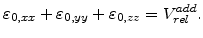
The chemical reaction of silicon and oxygen causes a volume increase of about 125%, which leads to significant displacements in the material. If this volume increase is only partially prevented, mechanical stress is built up in the materials. In order to calculate these displacements and stresses a mechanical modeling is needed.

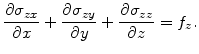
In general, every three-dimensional mechanical problem can be described by the stress equilibrium relations [70]

$$\frac{\partial \sigma_{xx}}{\partial x}+ \frac{\partial \sigma_{xy}}{\partial y}+ \frac{\partial \sigma_{xz}}{\partial z}= f_x,$$

$$\frac{\partial \sigma_{yx}}{\partial x}+ \frac{\partial \sigma_{yy}}{\partial y}+ \frac{\partial \sigma_{yz}}{\partial z}= f_y,$$ (3.14)

$$\frac{\partial \sigma_{zx}}{\partial x}+ \frac{\partial \sigma_{zy}}{\partial y}+ \frac{\partial \sigma_{zz}}{\partial z}= f_z.$$

During the oxidation process there are normally no external forces, because a volume increase caused by a chemical reaction, or a thermal expansion only lead to internal forces. Therefore, on the right-hand side of (3.14) the external forces are $f_x = f_y = f_z = 0$.

3.2.5.1 Elastic Mechanical Model

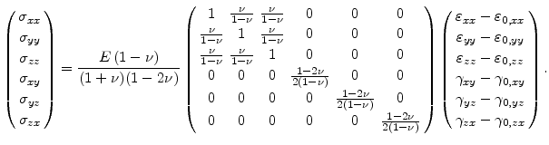
For linear elastic materials which are described by the Hook's law, the stress tensor $\tilde{\sigma}$ from (3.14) is given by

$$\tilde{\sigma} = \mathbf{D} (\tilde{\varepsilon} - \tilde{\varepsilon_0}) + \tilde{\sigma_0}.$$ (3.15)

Here $\mathbf{D}$ is the so-called material matrix. Furthermore, $\tilde{\varepsilon}$ is the strain tensor, $\tilde{\varepsilon_0}$ is the residual strain tensor, and $\tilde{\sigma_0}$ is the residual stress tensor.

For constructing the material matrix $\mathbf{D}$, the components of the stress tensor without residual stress and strain components can be expressed in Lame's form by [71]

$$\sigma_{ij}=\lambda \varepsilon_{kk} \delta_{ij}+2 \mu \varep... ..._{ij},%\begin{equation} x_0\cong\frac{B}{A}(t+\tau), %\clearpage \end{equation}$$ (3.16)

where $\varepsilon_{kk}$ is the trace of the strain tensor

$$\varepsilon_{kk}=\varepsilon_{xx}+\varepsilon_{yy}+\varepsilon_{zz},$$ (3.17)

$\delta_{ij}$ is the Kronecker symbol

$$\delta_{ij}=\left\{ \begin{array}{ll} 0 & \textrm{for } \mathrm{i\neq j} 1 & \textrm{for } \mathrm{i=j} \end{array}, \right.$$ (3.18)

and $\lambda$ and $\mu$ are the so-called Lame's constants

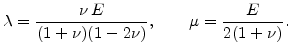$$\lambda=\frac{\nu E}{(1+\nu)(1-2\nu)}, \qquad \mu=\frac{E}{2(1+\nu)}.$$ (3.19)

Thereby $E$ is the Young modulus and $\nu$ is the Poisson ratio. Note, the often used shear modulus $G$ is identical with Lame's constant $\mu$.

The strain tensor is

$$\tilde{\varepsilon}= \left[ \begin{array}{ccc} \varepsilon_{xx} &... ...\gamma_{zx} & \frac{1}{2}\gamma_{zy} & \varepsilon_{zz} \end{array} \right].$$ (3.20)

The elements $\varepsilon_{ii}$ are the first derivatives of the displacements $u_{i}$ so that

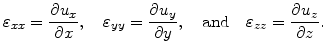$$\varepsilon_{xx}= \frac{\partial u_{x}}{\partial x}, \quad \varep... ..., \quad \mathrm{and} \quad \varepsilon_{zz}= \frac{\partial u_{z}}{\partial z}.$$ (3.21)

The shear strain components $2\varepsilon_{ij}= \gamma_{ij}$ are given by [72]

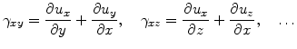$$\gamma_{xy}= \frac{\partial u_{x}}{\partial y}+\frac{\partial u_{... ...rac{\partial u_{x}}{\partial z}+\frac{\partial u_{z}}{\partial x}, \quad \ldots$$ (3.22)

If an isotropic material is assumed, the strain tensor is symmetric due to

$$\varepsilon_{xy}=\varepsilon_{yx}, \quad \varepsilon_{xz}=\varepsilon_{zx}, \quad \mathrm{and} \quad \varepsilon_{yz}=\varepsilon_{zy},$$ (3.23)

which means that there are only six different values.

Assuming an isotropic material and after constructing $\mathbf{D}$ with the help of (3.16), the stress tensor without residual stress, can be rewritten in the form

$$\left( \begin{array}{c} \sigma_{xx} \sigma_{yy} \sigma_{zz}\\... ... \gamma_{yz}-\gamma_{0,yz} \gamma_{zx}-\gamma_{0,zx} \end{array} \right).$$ (3.24)

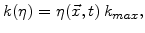
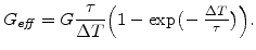
3.2.5.2 Visco-Elastic Mechanical Model

The material behavior of oxide and nitride are more realistically described with a visco-elastic model [73,74], especially with a so-called Maxwell element (see Fig. 3.3), which consists of a spring and a dashpot in series. The characteristics of such a Maxwell element is that it takes the stress relaxation and the stress history into account. Also the actual stress is influenced from both, the strain and the strain rate, and, therefore, the stress is a function of time. The Maxwell element can be mathematically formulated with

$$\frac{d\varepsilon}{dt} - \Big(\frac{d\sigma}{dt}\frac{1}{G}+ \frac{\sigma}{\gamma}\Big)=0,$$ (3.25)

where $G$ is the shear modulus and $\gamma$ is the (shear) viscosity.

Figure 3.3: Maxwell element: a spring and a dashpot in series.

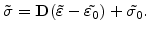
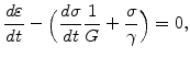
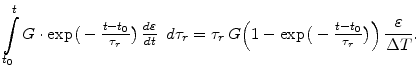
The analytical solution of (3.25) for the temporal stress evolution as a function of the strain velocity is

$$\sigma(t)=\sigma_0\cdot\mathrm{exp}\big(-\frac{{}_{t-t_0}}{{}^{\t... ...c{{}_{t-t_0}}{{}^{\tau_r}}\big) \frac{{}_{d\varepsilon}}{{}^{dt}}\; d\tau_r,$$ (3.26)

where $\sigma_0$ is the initial stress at time $t_0$ and $\tau_r$ is the Maxwellian relaxation time constant

$$\tau_r=\frac{\gamma}{G}.$$ (3.27)

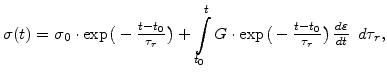
In (3.26) the first term shows that the initial stress relaxes exponentially with time. The evaluation of the integral part leads to

$$\int_{t_0}^t G\cdot\mathrm{exp}\big(-\frac{{}_{t-t_0}}{{}^{\tau_r... ...g(-\frac{{}_{t-t_0}}{{}^{\tau_r}}\big)\Big) \frac{{}_{d\varepsilon}}{{}^{dt}}.$$ (3.28)

The visco-elastic model is based on the idea that the dilatational components of the stress, which involve the volumetric expansion or compression, and the deviatoric components which only include the shape modification, can be decoupled [75]. For this purpose the material matrix $\mathbf{D}$ from (3.24) can be split in a dilatation and a deviatoric part [76]

$$\mathbf{D}=\mathbf{D}_{dil}+\mathbf{D}_{dev}= \left(H\left[ \begi... ...om{-}0 &\phantom{-}0 &\phantom{-}0 &\phantom{-}1 \end{array} \right] \right).$$ (3.29)

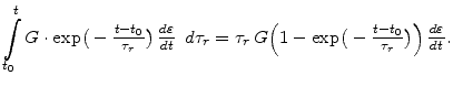
Here $H$ is the bulk modulus

$$H= \frac{E}{3(1-2\nu)},$$ (3.30)

and $G_\mathit{eff}$ is the so-called effective shear modulus which is in the elastic case the same as the standard shear modulus

$$G_\mathit{eff} = G = \frac{E}{2(1+\nu)}.$$ (3.31)

In Maxwell's model the dilatation part is assumed purely elastic, while the deviatoric part is modeled by the Maxwell element. In order to find an uncomplicated Maxwell formulation for the deviatoric part in (3.29), it can be assumed in (3.28) that for a short time period $\Delta T$ the strain velocity can be kept constant

$$\frac{d\varepsilon}{dt}=\frac{\varepsilon}{\Delta T},$$ (3.32)

so that (3.28) can be expressed in the form

$$\int_{t_0}^t G\cdot\mathrm{exp}\big(-\frac{{}_{t-t_0}}{{}^{\tau_r... ...}_{t-t_0}}{{}^{\tau_r}}\big)\Big) \frac{\varepsilon}{\Delta T}. \vspace*{-1mm}$$ (3.33)

So in the visco-elastic case $G_\mathit{eff}$ can be written in the form [77,78]

$$G_\mathit{eff} = G \frac{{\tau}}{{\Delta T}}\Big(1-\mathrm{exp}\big(\!-\frac{{}_{\Delta T}}{{}^{\tau}}\big)\Big).$$ (3.34)

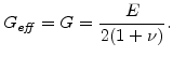
This relationship shows that the Maxwell visco-elasticity can be expressed by an effective shear modulus $G_\mathit{eff}$ in the deviatoric part of the material matrix $\mathbf{D}$ (3.24). This means that the only difference in the mechanical model between the elastic and visco-elastic case is the different $G_\mathit{eff}$ in the material matrix $\mathbf{D}$. So $\mathbf{D}$ depends in the elastic case only on Young's modulus $E$ and the Poisson ratio $\mathrm{\nu}$, and in the visco-elastic case additionally on the Maxwellian relaxation time $\tau$.

3.2.5.3 Volume Increase and Mechanics

A very important aspect in the oxidation model is, how the volume increase during oxidation can be brought in relation with the mechanical problem. In three dimensions a volume expansion can be formulated with

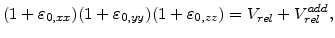$$(1+\varepsilon_{0,xx})(1+\varepsilon_{0,yy})(1+\varepsilon_{0,zz})=V_{rel}+V^{add}_{rel},$$ (3.35)

where $V_{rel}$ is the normalized volume before expansion and thus $V_{rel}$ is always 1.

By assuming that the volume expansion and the strain is small, the strain terms $\varepsilon_{0,ii}\cdot\varepsilon_{0,jj}$ can be neglected ($i$ and $j$ stands for $x$, $y$ or $z$), because they are much smaller than the terms $\varepsilon_{0,ii}$. Therefore, with the start volume $V_{rel}=1$, (3.35) can be reduced to the form

$$\varepsilon_{0,xx}+\varepsilon_{0,yy}+\varepsilon_{0,zz}=V^{add}_{rel}.$$ (3.36)

The components $\varepsilon_{0,ii}$ of the residual strain tensor $\tilde{\varepsilon_0}$ are linearly proportional to the normalized additional volume as calculated in (3.8)

$$\varepsilon_{0,ii}=\frac{{}_1}{{}^3}V^{add}_{rel},$$ (3.37)

which loads the mechanical problem (3.15) for calculating the displacements and stresses.