A look to the model (see Section 3.2.1) shows that there are three available parameters, namely the diffusion coefficient ![]() , the maximal possible strength of the spatial sink
, the maximal possible strength of the spatial sink ![]() , and the oxidant concentration
, and the oxidant concentration ![]() at surfaces which have contact to the oxidizing atmosphere. As displayed in (3.9) and (7.1) the diffusion coefficient has a physical background. It is temperature and stress dependent and its real physical value can be determined correctly. Therefore to use
at surfaces which have contact to the oxidizing atmosphere. As displayed in (3.9) and (7.1) the diffusion coefficient has a physical background. It is temperature and stress dependent and its real physical value can be determined correctly. Therefore to use ![]() for calibration is not appropriate.
for calibration is not appropriate.
The next parameter ![]() has more mathematical and modeling origin, but it is also not an optimal paramenter for calibration. At first the thickness of the reaction layer changes with
has more mathematical and modeling origin, but it is also not an optimal paramenter for calibration. At first the thickness of the reaction layer changes with ![]() , because it is inversely proportional to
, because it is inversely proportional to ![]() (see Section 3.2.4). This can be a problem for small
(see Section 3.2.4). This can be a problem for small ![]() values which lead to thick reaction layers.
values which lead to thick reaction layers.
For a better understanding of the second trouble with large ![]() values the following is worth mentioning: Simulations have shown that with regard to the finite elements for the value of
values the following is worth mentioning: Simulations have shown that with regard to the finite elements for the value of ![]() the following choice is reasonable
the following choice is reasonable
Due to the mesh dependence of ![]() its variation is limited. In the experiments it was found out that the value of
its variation is limited. In the experiments it was found out that the value of ![]() can not be increased arbitrarily. For larger values than suggested in (6.4) the numerical formulation becomes instable. In contrast to this, small
can not be increased arbitrarily. For larger values than suggested in (6.4) the numerical formulation becomes instable. In contrast to this, small ![]() values are not a problem. Therefore,
values are not a problem. Therefore, ![]() is not a suitable parameter for the model calibration of a potentially because of thick reaction layer (small value) and numerical instability (large value).
is not a suitable parameter for the model calibration of a potentially because of thick reaction layer (small value) and numerical instability (large value).
After excluding two of the three parameters, the last parameter which is the surface oxidant concentration ![]() is investigated. On surfaces which have contact with the oxidizing atmosphere the oxidant concentration is used as a Dirichlet boundary condition. The key idea is to modify
is investigated. On surfaces which have contact with the oxidizing atmosphere the oxidant concentration is used as a Dirichlet boundary condition. The key idea is to modify ![]() in order to calibrate the oxide thickness of the simulated oxidation process over time for different oxidation conditions. From the physical aspect a higher surface oxidant concentration means that a larger number of oxidants diffuse to the Si/SiO
in order to calibrate the oxide thickness of the simulated oxidation process over time for different oxidation conditions. From the physical aspect a higher surface oxidant concentration means that a larger number of oxidants diffuse to the Si/SiO![]() -interface and react with silicon, which results in a faster oxidation rate.
-interface and react with silicon, which results in a faster oxidation rate.
It was found with experiments that the best results are obtained if ![]() consists of a constant part
consists of a constant part
![]() and an
and an
![]() -dependent part
-dependent part
![]() so that the effective surface concentration can be written as a function of
so that the effective surface concentration can be written as a function of ![]()
As example for the above described calibration concept a (111) oriented and 0.4![]() m height silicon block is wet oxidized and the oxide thickness over time for different temperatures is calibrated. The bottom surface is fixed, the lateral surfaces can only move vertically and on the upper surface a free mechanical boundary condition is applied. Only the upper surface of the body has contact with the oxidizing atmosphere. The oxide thickness is measured between the upper surface and the
m height silicon block is wet oxidized and the oxide thickness over time for different temperatures is calibrated. The bottom surface is fixed, the lateral surfaces can only move vertically and on the upper surface a free mechanical boundary condition is applied. Only the upper surface of the body has contact with the oxidizing atmosphere. The oxide thickness is measured between the upper surface and the ![]() -level of 0.5.
-level of 0.5.
In the calibration process the values of the parameters ![]() ,
, ![]() , and
, and ![]() are determined with the help of the in-house tool SIESTA (Simulation Environment for Semiconductor Technology Analysis) [108], so that the thickness values of the simulated oxide layers agree with the calculated physical reference values up to approximately 500nm at any time for a temperature range of 900-1100
are determined with the help of the in-house tool SIESTA (Simulation Environment for Semiconductor Technology Analysis) [108], so that the thickness values of the simulated oxide layers agree with the calculated physical reference values up to approximately 500nm at any time for a temperature range of 900-1100![]() C.
The temperature dependent diffusion coefficient
C.
The temperature dependent diffusion coefficient ![]() is calculated as explained in (3.13). The other two model parameter
is calculated as explained in (3.13). The other two model parameter
![]() and
and
![]() are kept constant over the whole temperature range.
are kept constant over the whole temperature range.
It was found that in case of wet oxidation the value of the parameter
![]() in (6.5) can be hold constant for the temperature range of T=900-1100
in (6.5) can be hold constant for the temperature range of T=900-1100![]() C. Furthermore, the experiments show that the parameter
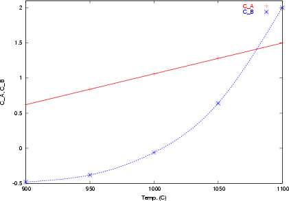
C. Furthermore, the experiments show that the parameter ![]() can be brought to a linear and the parameter
can be brought to a linear and the parameter ![]() can be brought to a parabolic dependence on temperature, which is described by
can be brought to a parabolic dependence on temperature, which is described by
![\includegraphics[width=0.52\linewidth,bb= 38 52 727 548, clip]{curv-calib/900C_3/900plota}](img842.png)
![\includegraphics[width=0.52\linewidth,bb= 38 52 722 548, clip]{curv-calib/1000C_3/plot2-1000C}](img843.png)
![\includegraphics[width=0.52\linewidth,bb= 38 52 722 548, clip]{curv-calib/1100C_2/plot1100}](img844.png)