In this chapter a short introduction to the theory of stress and strain in elastic bodies is given. To improve the performance of FBMC simulations it is important to take advantage of the symmetry properties of the band structure. Therefore, the symmetry properties of the reciprocal diamond lattice are investigated in detail for several strain conditions.
To keep a body in static equilibrium the sum of all forces acting on it must be
zero. If a small cubicle volume as depicted in Figure 2.1 of the body
is considered, forces
![]() act on the surfaces
act on the surfaces
![]() .
The index i indicates one of the surface planes. The stress vector
.
The index i indicates one of the surface planes. The stress vector
![]() is then
defined as the limit [Bir74]
is then
defined as the limit [Bir74]
 |
(2.1) |
As depicted in Figure 2.1, each of the three stress vectors can be decomposed into two components within the plane, the so called shear stress components, and one normal component. The total number of six shear stress components and three normal stress components can be lumped together into the stress tensor
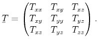 |
(2.2) |
| (2.3) |
 |
(2.4) |
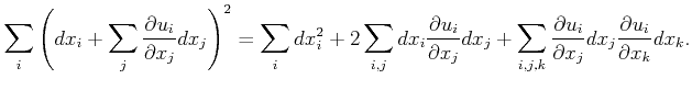
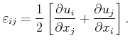
 |
||
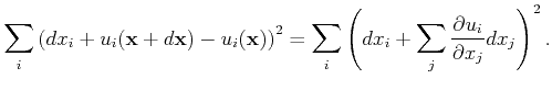
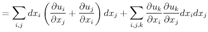
![$\displaystyle = \sum_{i,j} dx_i\left[ { \left(\frac{\partial u_i}{\partial x_j}...
...\frac{\partial u_k}{\partial x_i }\frac{\partial u_k}{\partial x_j}}\right]dx_j$](img117.png) |
||
 |
(2.6) |
 holds,
the second order term in (2.7) can be neglected. This simplifies the resulting tensor components to
holds,
the second order term in (2.7) can be neglected. This simplifies the resulting tensor components to
 |
(2.9) |
| (2.10) |
| (2.11) |
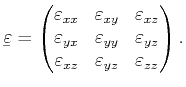
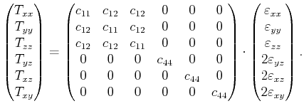
The number of independent components in the elastic stiffness tensor is
further reduced by symmetry properties of the considered crystal
[Kittel96]. For cubic semiconductors such as Si, Ge or GaAs, the elastic stiffness tensor
contains only three independent components,
![]() , and
, and ![]() , which
lead to a stress-strain relation of the form
, which
lead to a stress-strain relation of the form
|
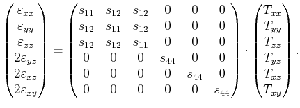
In the case that the stresses are known, the values for the strains have to be
determined by inversion of (2.12). With the introduction of the elastic
compliance tensor ![]() , the inverted equation reads
, the inverted equation reads
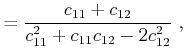 |
(2.16) | |
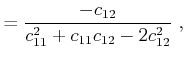 |
(2.17) | |
 |
(2.18) |
To specify directions and planes in a crystal the Miller index notation is
commonly used [Ashcroft76,Kittel96]. The Miller indices of a plane are
defined in the following way: In a first step three lattice vectors, which form
the axis of the crystallographic coordinate system have to be found. In cubic
crystal systems, the lattice vectors are chosen along the edges of the
crystallographic unit cell. Second the points where a crystal plane intercepts
the axes are derived and their coordinates are transformed into fractional
coordinates by dividing by the respective cell dimension. In a last step the
Miller indices are obtained as the reciprocals of the fractional
coordinates. For a cubic crystal they are given as a triplet of integer values
![]() . A Miller index 0
indicates a plane parallel to the respective
axis. Negative indices are defined by a bar written over the number. To denote
all planes equivalent by symmetry, the notation
. A Miller index 0
indicates a plane parallel to the respective
axis. Negative indices are defined by a bar written over the number. To denote
all planes equivalent by symmetry, the notation
![]() is used.
is used.
It is also common to indicate directions in the basis of the
lattice vectors by Miller indices with square brackets like in ![]() . The
notation
. The
notation
![]() is used to indicate all directions that are
equivalent to
is used to indicate all directions that are
equivalent to ![]() by crystal symmetry.
by crystal symmetry.
Figure 2.2 depicts the Miller notation for several planes in the cubic system. The Miller indices of a plane coincide with those of the direction perpendicular to the plane.
Uniaxial stress applied along symmetry directions of the cubical crystal is of technological importance since it is preferably used in actual devices. The stress and strain tensors in the principal coordinate system of the crystal are given in the following for uniaxial stress of magnitude S applied along [100], [110], [111] and [120] directions, respectively. Here, the strain tensors are calculated by inserting the corresponding stress tensors in (2.15).
![$\displaystyle \ensuremath{{\underaccent{\bar}{T}}}_{[100]} = S \begin{pmatrix}1...
...\begin{pmatrix}s_{11} & 0 & 0 0 & s_{12} & 0 0 & 0 & s_{12} \end{pmatrix}$](img142.png) |
![$\displaystyle \ensuremath{{\underaccent{\bar}{T}}}_{[110]} = \frac {S} {2} \beg...
...& s_{44}/2 & 0 s_{44} /2 & s_{11}+s_{12} & 0 0 & 0 & s_{12} \end{pmatrix}$](img143.png) |
Biaxial strain can be introduced in Si by epitaxially growing a Si layer on an
SiGe substrate, which features a different lattice constant. The Si layer adjusts to
the lattice constant of the SiGe substrate and becomes globally biaxially
strained. If the interface is a ![]() -plane the strain
tensor reads [Hinckley90]
-plane the strain
tensor reads [Hinckley90]
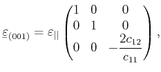 |
(2.20) |
 |
(2.21) |
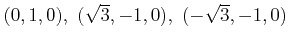
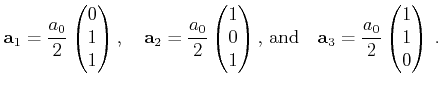
Figure 2.4 depicts the structure of the diamond
lattice, which is the lattice of group IV semiconductors such as Si and Ge. The
basis consists of two atoms at ![]() and
and
![]() and the basis vectors
and the basis vectors ![]() ,
, ![]() and
and ![]() . The lattice can also be described as two inter-penetrating face centered
cubic (fcc) lattices, one displaced from the other by a translation of
. The lattice can also be described as two inter-penetrating face centered
cubic (fcc) lattices, one displaced from the other by a translation of
![]() along a body diagonal.
along a body diagonal.
![\includegraphics[width=3.5in]{inkscape/DiamondLattice_g.eps}](img157.png)
|
For group IV semiconductors the two basis atoms are identical, whereas for III-V semiconductors such as GaAs, AlsAs, InAs, or InP the basis atoms are different and the structure is called the zinc-blende structure.
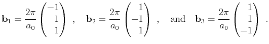
The basis vectors of the Bravais lattice read
| (2.23) |
Generally, applying strain to a crystal reduces its symmetry. The basis vectors
![]() of the strained Bravais lattice can be directly obtained by a
transformation of the vectors
of the strained Bravais lattice can be directly obtained by a
transformation of the vectors ![]() of the unstrained
crystal [Bir74]
of the unstrained
crystal [Bir74]
| (2.26) |
To describe the lattice symmetry properties on a more formal basis a definition of the possible point operations is needed:
E unity operationwhere
nclockwise rotation of angle
around axis

ncounter-clockwise rotation of angle
I inversion
clockwise rotation of angle
counter-clockwise rotation of angle
 =


 =


 =


 =


 =
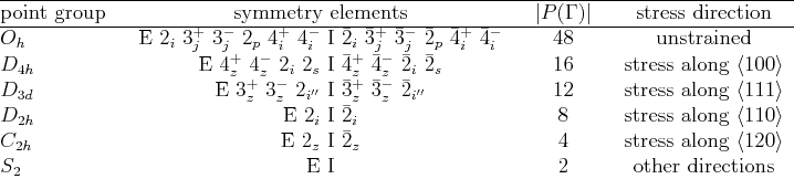
Table 2.2 [Yu03] lists the resulting point groups in
Schönfließ notation when applying strain to the diamond
lattice. Starting point is the unstrained diamond structure denoted by
![]() .
.
![]() denotes the number of elements of the point group which is
48 for
denotes the number of elements of the point group which is
48 for ![]() and is decreased under strain as indicated in the table.
and is decreased under strain as indicated in the table.
 |
 |
(2.28) |
The unit cell of the reciprocal lattice is the Brillouin zone. It contains all points nearest to one enclosed lattice point. Due to periodicity of the reciprocal lattice only the first Brillouin zone has to be considered for band structure calculation. The shape of the first Brillouin zone is determined by the boundary faces
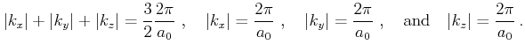 |
(2.30) |
The volume for band structure calculation can be further reduced by taking into account that the symmetry operations for the reciprocal lattice are the same as for the Bravais lattice. Therefore the symmetry elements given in Table 2.2 can be directly applied to the reciprocal lattice cell. The smallest possible domain in the Brillouin zone is termed the irreducible wedge. Figure 2.5 depicts the first Brillouin zone highlighting the irreducible wedge as well as one octant.
Figure 2.6 shows one octant of the Brillouin zone and a detailed view of the irreducible wedge with the location of some symmetry points as they are usually named in literature.
Biaxial strain applied in a ![]() plane of a cubic lattice transforms the
cell from
plane of a cubic lattice transforms the
cell from ![]() to the
to the ![]() symmetry, a member of the tetragonal crystal
class [Bir74]. The same symmetry reduction is observed, if uniaxial strain
along a fourfold axis
symmetry, a member of the tetragonal crystal
class [Bir74]. The same symmetry reduction is observed, if uniaxial strain
along a fourfold axis ![]() is applied.
The point group
is applied.
The point group ![]() has 16 remaining symmetry elements. The symmetry
operations maintain invariance of the energy bands under reflections
has 16 remaining symmetry elements. The symmetry
operations maintain invariance of the energy bands under reflections
The cube of the crystal class ![]() is converted to a parallelepiped of the
orthorhombic system belonging to
is converted to a parallelepiped of the
orthorhombic system belonging to ![]() when uniaxial stress is applied along
when uniaxial stress is applied along
![]() or when biaxial strain is applied in a
or when biaxial strain is applied in a ![]() plane.
Equation (2.19) exhibits the form of the strain tensor [Bir74] which
includes off-diagonal elements. As a result the unit cube is sheared and the
angles between the basis vectors are altered.
plane.
Equation (2.19) exhibits the form of the strain tensor [Bir74] which
includes off-diagonal elements. As a result the unit cube is sheared and the
angles between the basis vectors are altered.
The ![]() group has only eight symmetry elements (given in
Table 2.2). A possible irreducible wedge with a volume of
group has only eight symmetry elements (given in
Table 2.2). A possible irreducible wedge with a volume of
![]() is depicted in Figure 2.9. The irreducible wedge
is any of the eight octants of the Brillouin zone.
It should be noted that the
is depicted in Figure 2.9. The irreducible wedge
is any of the eight octants of the Brillouin zone.
It should be noted that the ![]() group can also be reached by applying
strain to the
group can also be reached by applying
strain to the ![]() class along two of the three fourfold axes
class along two of the three fourfold axes ![]() . In this case, the strain tensor consists of three different diagonal
elements
. In this case, the strain tensor consists of three different diagonal
elements
![]() ,
,
![]() , and
, and
![]() and vanishing off-diagonal
components.
and vanishing off-diagonal
components.
Under arbitrary stress - that is stress along directions other than those given
in Table 2.2 - no rotational symmetries remain. The crystal
is invariant only under inversion and therefore a member of the crystal class
![]() . In this case half of the Brillouin zone must be chosen as the irreducible volume for band
structure calculation and for the transport simulation.
. In this case half of the Brillouin zone must be chosen as the irreducible volume for band
structure calculation and for the transport simulation.
As illustrated in the last section, only the irreducible wedge is needed as the actual simulation domain. Mapping a carrier back to the domain of the irreducible wedge is more complicated as a coordinate transformation is necessary after applying equation (2.35) and every possible shape of the irreducible wedge demands for its own set of transformation rules.
To keep the code simple only two sizes of the simulation domain are implemented in the simulator: if the irreducible wedge fits into the first octant then the first octant is chosen as the domain, if it exceeds the first octant one half of the Brillouin zone is chosen. Since these domains can be larger then the irreducible wedge it may be necessary to extend the original band structure data by permutation.
In the case of the first octant as the simulation domain the octants are
numbered as shown in Figure 2.10. If the carrier crosses the Brillouin
zone border in a first step it is mapped back by subtraction of a lattice
vector. In a second step it is mapped into the first octant by a coordinate
transformation. This coordinate transformation is simply realized by a set of
mirror operations as shown in Table 2.3. The table entries indicate
which of the coordinates ![]() ,
, ![]() and
and ![]() have to be mirrored for a
specific transition from one octant to another. The transformation is applied
to the particle
have to be mirrored for a
specific transition from one octant to another. The transformation is applied
to the particle
![]() -vector and to the force vector
(see also equation of motion (3.3)).
-vector and to the force vector
(see also equation of motion (3.3)).
If the carrier is crossing a border to another octant within the Brillouin zone, the mirror operations are applied to map it back to the first octant.
If one half of the Brillouin zone is used as the simulation
domain there is only one mirroring operation: all three coordinates of the
![]() -vector and the force vector
are mirrored if a transition from one halfspace to the other occurs.
-vector and the force vector
are mirrored if a transition from one halfspace to the other occurs.
![\includegraphics[scale=1.1, clip]{inkscape/stressExp2.eps}](img105.png)
![$\displaystyle \varepsilon _{ij} = \frac{1}{2}\left[\frac{\partial u_i}{\partial...
...rac{\partial u_k}{\partial x_i }\frac{\partial u_k}{\partial x_j} } \right] .$](img119.png)
![\includegraphics[scale=3.4, clip]{inkscape_fig/miller.fig3.eps}](img141.png)
![$\displaystyle \ensuremath{{\underaccent{\bar}{T}}}_{[111]} = \frac {S} {3} \beg...
...{11}+2s_{12} & s_{44}/2 s_{44} /2 & s_{44} /2 & s_{11}+2s_{12} \end{pmatrix}$](img144.png)
![$\displaystyle \ensuremath{{\underaccent{\bar}{T}}}_{[120]} = \frac {S} {5} \beg...
...{44} & 0 s_{44} & s_{12}\!+\!4s_{11} & 0 0 & 0 & 5 s_{12} \end{pmatrix}$](img145.png)
![\includegraphics[width=1\linewidth]{figures//Bravais_table.epsi}](img151.png)
![\includegraphics[width=4.15in]{inkscape/brillouin3.eps2}](img193.png)
![\includegraphics[width=4.15in]{inkscape/Octant3.eps}](img194.png)
![\includegraphics[width=4in]{xmgrace-files/Si_bandstructure3.eps}](img200.png)
![\includegraphics[width=3.6in, clip]{figures/sispad_100_2.eps2}](img207.png)
![\includegraphics[width=3.6in, clip]{figures/sispad_110_2.eps2}](img208.png)
![\includegraphics[width=0.7\linewidth]{figures/octants.svg.eps}](img221.png)