Previous: 2.3.2 Grid Generation Up: 2. Three-Dimensional Device Simulation Next: 2.5 Control System
For the discretization [73] of the differential equations the
Finite-Boxes method (box integration method) is used. It uses a grid
consisting of points and lines where each point ![]() is assigned its
Voronoi box
is assigned its
Voronoi box
![]() (see
Section 2.3.1) which is defined as
its corresponding part of the simulation area. All boxes together form the
whole simulation area
(see
Section 2.3.1) which is defined as
its corresponding part of the simulation area. All boxes together form the
whole simulation area ![]() .
.
All points and therefore all the boxes are numbered. Boxes that touch each other are connected by lines. As the Voronoi diagram and the grid are dual, the inverse definition is valid too: if points are connected by lines, the corresponding boxes touch each other.
Adjacent boxes are called neighboring boxes. A box can have an arbitrary number of neighboring boxes. For the discretization an information like ``the number of the next neighboring point in order'' or ``the number of the neighbor of two neighboring points'' is not available and not needed. The discretization scheme in Minimos-NT uses unstructured neighborhood information. The advantage of this procedure is that the discretization scheme is independent of the type of the grid used. This enables to apply any kind of grid, because no special kind of grid is taken for granted. Nevertheless, the grids have to meet the criterions discussed in Section 2.3.
The unstructured neighborhood information consists of the following data:

|
|
|
|
The basic semiconductor equations consist of Poisson's equation, the continuity equation for electrons and holes and the equations for the current density for electrons and holes. The current relations (2.4) and (2.5) are given for the drift-diffusion case. This set of equations was first presented by Van Roosbroeck [20] in 1950.
Equation (2.1) is derived from the third Maxwell equation for the dielectric displacement under assumption of a static magnetic and electric field. The equations (2.2) and (2.3) are derived from the first and the third Maxwell equations. The assumption made is that only the mobile charge represented by electrons and holes are time variant. By introducing a generation/recombination term the equations can be separated into to parts, one for electrons and one for holes as shown above. By superpositioning the current given by Ohm's law and the particle flux density for each carrier type the drift-diffusion current relations for electrons (2.4) and holes (2.5) are derived [19,73,88].
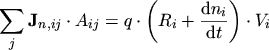
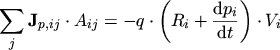
To discretize Poisson's equation (2.1) the third Maxwell
equation is used. For the equations (2.1),
(2.2), and (2.3) Gaussian's law is
applied by integrating the equations over a Voronoi box
![]() of a point
of a point
![]() . By approximizing the integrals with sums over all neighboring
points
. By approximizing the integrals with sums over all neighboring
points ![]() the following equations are obtained:
the following equations are obtained:
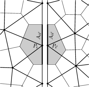
![]() is the volume of the Voronoi box
is the volume of the Voronoi box
![]() and
and
![]() is the
interface area between the two adjacent Voronoi boxes
is the
interface area between the two adjacent Voronoi boxes
![]() and
and
![]() .
.
![]() ,
,
![]() , and
, and
![]() are the projections of
are the projections of
![]() ,
,
![]() , and
, and
![]() on the grid line between
on the grid line between ![]() and
and
![]() in the middle of the line. Now, only a suitable discretization of
these quantities has to be found.
in the middle of the line. Now, only a suitable discretization of
these quantities has to be found.
An approximation of
![]() can be found where
can be found where
![]() denotes the
distance between the two neighboring points
denotes the
distance between the two neighboring points ![]() and
and ![]() :
:
Great care has to be taken for the discretization of
![]() and
and
![]() given by (2.4) and (2.5).
This is because the quantities
given by (2.4) and (2.5).
This is because the quantities ![]() and
and ![]() change exponentially between two
grid points. Using a discretization scheme in analogy to
(2.9) would require an extremely dense mesh. The
method of Scharfetter-Gummel [104] has been proven to be a useful
discretization of the current density. Solving the equations
[88] then leads to
change exponentially between two
grid points. Using a discretization scheme in analogy to
(2.9) would require an extremely dense mesh. The
method of Scharfetter-Gummel [104] has been proven to be a useful
discretization of the current density. Solving the equations
[88] then leads to
with
and the Bernoulli function
Both the drift diffusion model and the hydrodynamic model can be obtained from the Boltzmann equation
where ![]() is
is ![]() for electrons and
for electrons and ![]() for holes.
for holes.
![]() is the electric
field,
is the electric
field,
![]() is the group velocity and
is the group velocity and
![]() the collision operator. A more
general way is given by the solution using
the collision operator. A more
general way is given by the solution using ![]() moments instead of up to
moments instead of up to ![]() for
the drift diffusion model or
for
the drift diffusion model or ![]() for the hydrodynamic model
[105]. Thereby the physically motivated weight functions
for the hydrodynamic model
[105]. Thereby the physically motivated weight functions
are used to define the moments of the distribution function
| (2.15) |
By integrating over the ![]() -space the closing condition
-space the closing condition
| (2.16) |
is used where ![]() is the carrier concentration (
is the carrier concentration (![]() or
or ![]() ) with
) with
![]() and
and ![]() denotes a moment which has to be modeled properly to
obtain the following set of equations [105]:
denotes a moment which has to be modeled properly to
obtain the following set of equations [105]:
| (2.17) | ||
| (2.18) |
| (2.19) | ||
| (2.20) |
| (2.21) | ||
| (2.22) |
For the discretization of the fluxes
![]() ,
,
![]() , and
, and
![]() the projected flux between two grid points is assumed constant and the
temperature for each flux
the projected flux between two grid points is assumed constant and the
temperature for each flux ![]() is interpolated linearly. The
Scharfetter-Gummel type discretization for each flux
is interpolated linearly. The
Scharfetter-Gummel type discretization for each flux ![]() then gives
then gives
| (2.23) |
| (2.24) |
For the discretization the inner products
![]() of the
fluxes are written as
of the
fluxes are written as
| (2.25) |
which is discretized using the standard box integration method [19,73,88].
It is important to note, that the whole discretization is independent from the dimensionality of the device. Only the neighborhood information is needed which has been depicted at the beginning of this section. As Minimos-NT has been expanded to a three-dimensional simulator this discretization scheme did not change. Only the vectors had to support three-dimensional coordinates. In the discretization scheme above only the drift-diffusion case is shown. The hydrodynamic case, the discretization of energy-balance and other equations is shown in [73,88,106] in detail.
Vector quantities are only needed in some models. In the discretization shown
above the vector quantities have been projected on the grid line between
![]() and
and ![]() . Therefore only the projected component of the
vector contributes to the equations. It is not possible to calculate the full
vector because the vector component orthogonal to the grid line is not known.
. Therefore only the projected component of the
vector contributes to the equations. It is not possible to calculate the full
vector because the vector component orthogonal to the grid line is not known.
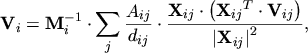
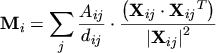
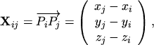
To fully determine a vector quantity on an arbitrary point in the simulation domain it is, therefore, necessary to analyze the vectors in all neighboring points. Moreover, a calculation scheme is necessary, which deals with unstructured neighborhood information only. Thus, the scheme shown in [73] has been extended to
where
![]() denotes a vector quantity at the point
denotes a vector quantity at the point ![]() and
and
![]() the vector quantity at the middle of the grid line between
the vector quantity at the middle of the grid line between ![]() and
and
![]() .
.
![]() is a matrix containing the weight of the neighboring
points.
is a matrix containing the weight of the neighboring
points.
Since most of the equations and models contain vectors it has to be guaranteed that the formulas work for the one-, two, and three-dimensional case. Different implementations for different dimensionalities are not convenient and are a source of errors. Therefore, the quantities, the equations, and the representation of the device have to be implemented in a self-consistent way.
Robert Klima 2003-02-06