4.1.3 Shape Function

The shape function is the function which interpolates the solution between the discrete values obtained at the mesh nodes. Therefore, appropriate functions have to be used and, as already mentioned, low order polynomials are typically chosen as shape functions. In this work linear shape functions are used.

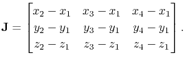
For three-dimensional finite element simulations it is convenient to discretize the simulation domain using tetrahedrons, as depicted in Figure 4.1. Thus, linear shape functions must be defined for each tetrahedron of the mesh, in order to apply the Galerkin method described in Section 4.1.1.

Figure 4.1: Finite element mesh of a three-dimensional interconnect structure discretized with tetrahedrons.

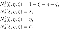
Consider a tetrahedron in a cartesian system as depicted in Figure 4.2(a). The linear shape function of the node $i$ has the form [153]

$$N_i(x,y,z) = a_i + b_i x + c_i y + d_i z,$$ (4.15)

where $i=1,...,4$. The coefficients, $a_i, b_i, c_i,$ and $d_i$ for each nodal basis function of the tetrahedral element can be calculated considering the condition [152]

$$N_j(\vec r_i) = \symKronecker,\qquad i,j=1,...,4.$$ (4.16)

As a result, a system of $4$ equations for the $4$ unknown coefficients is obtained. This procedure has to be repeated for all tetrahedrons of the mesh, so that the basis functions of all grid nodes are determined. Furthermore, in order to obtain the discrete system of equations (4.9), the shape functions have to be derived and integrated, as shown by (4.11) and (4.12).

Figure: Tetrahedral finite element. (a) Original coordinate system. (b) Transformed coordinate system.

(a)                                                                   (b)

The calculations can be significantly simplified by carring out a coordinate transformation. A tetrahedron in a transformed coordinate system is shown in Figure 4.2(b). Each point $(x,y,z)$ of the tetrahedron in the original coordinate system can be mapped to a corresponding point $(\xi,\eta,\zeta)$ in the transformed coordinate system [155]

$$x = x_1 + (x_2 - x_1)\xi + (x_3 - x_1)\eta + (x_4 - x_1)\zeta,$$

$$y = y_1 + (y_2 - y_1)\xi + (y_3 - y_1)\eta + (y_4 - y_1)\zeta,$$ (4.17)

$$z = z_1 + (z_2 - z_1)\xi + (z_3 - z_1)\eta + (z_4 - z_1)\zeta,$$

which in matrix form leads to the Jacobian matrix

$$\mathbf{J} = \begin{bmatrix}x_2-x_1 & x_3-x_1 & x_4-x_1\\ y_2-y_1 & y_3-y_1 & y_4-y_1\\ z_2-z_1 & z_3-z_1 & z_4-z_1\end{bmatrix}.$$ (4.18)

In this way, the nodal basis functions for the tetrahedron in the transformed coordinate system are given by [155]

$$\begin{aligned}&N_1^t(\xi,\eta,\zeta)= 1-\xi-\eta-\zeta,\\ &N_2... ...\eta,\zeta)= \eta,\\ &N_4^t(\xi,\eta,\zeta)= \zeta. \end{aligned}$$

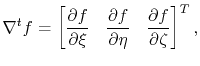
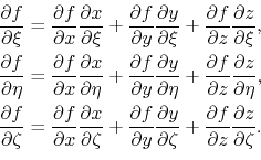
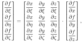
These shape functions are rather simple, so that the derivatives and integrals required for the finite element formulation can be readily evaluated in the transformed coordinate system. Given a function $f(x,y,z)$, the gradient in the transformed coordinates is of the form

$$\nabla^t f = \begin{bmatrix}\displaystyle\ensuremath{\frac{\parti... ...} &\displaystyle\ensuremath{\frac{\partial f}{\partial \zeta}} \end{bmatrix}^T,$$ (4.20)

where the derivatives are calculated via the chain rule by

$$\begin{aligned}&\ensuremath{\frac{\partial f}{\partial \xi}}=\e... ...z}}}\ensuremath{\frac{\partial z}{\partial \zeta}}. \end{aligned}$$

These equations can be expressed in matrix notation as

$$\begin{bmatrix}\displaystyle\ensuremath{\frac{\partial f}{\partia... ...playstyle\ensuremath{\ensuremath{\frac{\partial f}{\partial z}}} \end{bmatrix},$$ (4.22)

or

$$\nabla^t f = \mathbf{J}^T\ensuremath{\nabla{f}},$$ (4.23)

where $\mathbf{J}^T$ is the transpose of the Jacobian matrix. Thus, the gradient in the original coordinate system can be calculated using the transformed coordinate gradient by

$$\ensuremath{\nabla{f}} = \left(\mathbf{J}^T\right)^{-1}\nabla^t f = \mathbf{\Lambda}\nabla^t f,$$ (4.24)

where $\mathbf{\Lambda} = \left(\mathbf{J}^T\right)^{-1}$.

Performing such a coordinate transformation significantly simplifies the practical implementation of the FEM. The nodal shape functions in the transformed coordinates are fixed and known in advance, thus, it is not necessary to solve the system of equations formed by (4.15) and (4.16) for each element of the mesh. Only the Jacobian matrix has to be determined, and the required calculations for the finite element formulation can be easily evaluated.