


Next: 4.3 Simulation in FEDOS
Up: 4.2 Discretization of the
Previous: 4.2.3 Discretization of the
4.2.4 Discretization of the Mechanical Equations
The deformation in a three-dimensional body is expressed by the displacement field
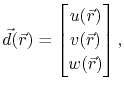 |
(4.54) |
where  ,
,  , and
, and  are the displacements in the x, y, and z direction, respectively.
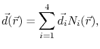
The displacement is discretized on a tetrahedral element as [151]
are the displacements in the x, y, and z direction, respectively.
The displacement is discretized on a tetrahedral element as [151]
 |
(4.55) |
which leads to the components discretization
 |
(4.56) |
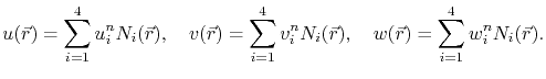
Applying this discretization in the strain-displacement relationship (3.79), the components of the strain tensor can be written as
 |
(4.57) |
where
 is the matrix of the derivatives of the shape functions for the node i [151]
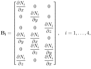 |
(4.58) |
and the displacement matrix
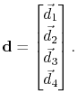 |
(4.59) |
Using (4.57), the stress-strain equation (3.81) can written as a function of the displacements according to
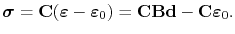 |
(4.60) |
Applying the principle of virtual work, the work of internal stresses on a continuous elastic body is given by [151]
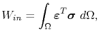 |
(4.61) |
where
 is the transposed strain tensor.
Combining (4.57), (4.60), and (4.61) the work on a finite element is written as
is the transposed strain tensor.
Combining (4.57), (4.60), and (4.61) the work on a finite element is written as
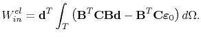 |
(4.62) |
From energy balance the internal work should be equal to the work done by external forces, i.e.
 , and, since during electromigration there are no external forces (
 ), one obtains
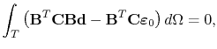 |
(4.63) |
or
 |
(4.64) |
which can be conveniently expressed as
 |
(4.65) |
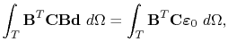
where
 |
(4.66) |
is the so-called stiffness matrix, and
 |
(4.67) |
is the internal force vector.
Equation (4.65) forms a linear system of equations of 12 equations with 12 unknowns (the three displacement components  ,
,  , and
, and  for each tetrahedron node).
The inelastic strain
for each tetrahedron node).
The inelastic strain
 determines the internal force vector according to the electromigration induced strain given by (3.78).
Next: 4.3 Simulation in FEDOS
Up: 4.2 Discretization of the
Previous: 4.2.3 Discretization of the
R. L. de Orio: Electromigration Modeling and Simulation