4.2.3 Discretization of the Vacancy Balance Equation

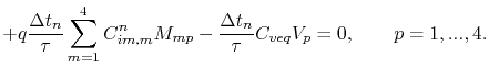
The combination of (3.74) with (3.75) and (3.76) yields the vacancy balance equation

$$\ensuremath{\ensuremath{\frac{\partial \CV}{\partial t}}} +\ensur... ...Factor\symAtomVol}{\kB\T}\CV\ensuremath{\nabla{\symHydStress}}\biggr) \right]}}$$

$$+\frac{1}{\symVacRelTime}\left(q\Cim - \Ceq\right) = 0,$$ (4.41)

for which the weak formulation of the form

$$\int_{\symDomain}\ensuremath{\ensuremath{\frac{\partial \CV}{\par... ...nsuremath{\cdot}\ensuremath{\nabla{\symShapeFun_p}}\right)\ d\symDomain \right.$$

$$- \left. \frac{\Q}{\kB\bar\T^2} \int_{\symDomain}\CV\left(\ensure... ...nsuremath{\cdot}\ensuremath{\nabla{\symShapeFun_p}}\right)\ d\symDomain \right]$$ (4.42)

$$+\int_{\symDomain}\frac{1}{\symVacRelTime}\left(q\Cim - \Ceq\right)\symShapeFun_p\ d\symDomain = 0, \quad p=1,...,N,$$

is obtained under the assumption of a Neumann boundary condition. Applying the electric potential and the temperature discretization, (4.29) and (4.36), respectively, together with

$$\CV^n = \ensuremath{\sum_{k=1}^{4}{C}}_{v,k}^n\symShapeFun_k(\vec r),$$ (4.43)

$$\symHydStress^n = \ensuremath{\sum_{l=1}^{4}{\symHydStress}}_l^n\symShapeFun_l(\vec r),$$ (4.44)

$$\Cim^n = \ensuremath{\sum_{m=1}^{4}{C}}_{im,m}^n\symShapeFun_m(\vec r),$$ (4.45)

and the backward Euler time discretization, the vacancy balance equation discretized in a single element is given by

$$\sum_{k=1}^{4} C_{v,k}^n \int_{T} \symShapeFun_k \symShapeFun_p\ ... ...n_k}}\ensuremath{\cdot}\ensuremath{\nabla{\symShapeFun_p}}\ d\symDomain \right.$$

$$+ \frac{\vert\Z\vert\ee}{\kB\bar\T} \sum_{i=1}^4\sum_{k=1}^4 \sym... ...th{\cdot}\ensuremath{\nabla{\symShapeFun_p}}\right) \symShapeFun_k\ d\symDomain$$

$$- \frac{\Q}{\kB\bar\T^2} \sum_{j=1}^4\sum_{k=1}^4 \T_j^n C_{v,k}^... ...th{\cdot}\ensuremath{\nabla{\symShapeFun_p}}\right) \symShapeFun_k\ d\symDomain$$ (4.46)

$$+ \left. \frac{\symVacRelFactor\symAtomVol}{\kB\bar\T} \sum_{l=1}... ...}\ensuremath{\nabla{\symShapeFun_p}}\right) \symShapeFun_k\ d\symDomain \right]$$

$$+ \frac{\Delta t_n}{\symVacRelTime} \left(q\sum_{m=1}^4 C_{im,m}^... ...symDomain - \Ceq\int_{T}\symShapeFun_p\ d\symDomain\right) = 0,\qquad p=1,...,4$$

under the assumption that $\symVacRelTime$, $q$, and $\Ceq$ are constant inside an element.

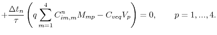
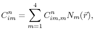
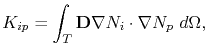
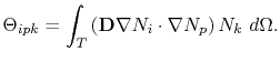
Using the shorthand notation (4.31), (4.38), (4.39), and

$$V_p = \int_{T} \symShapeFun_p\ d\symDomain = \det(\mathbf{J})\int_{0}^{1}\int_{0}^{1-\xi}\int_{0}^{1-\xi-\eta}\symShapeFun_p^t\ d\zeta d\eta d\xi,$$ (4.47)

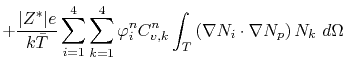
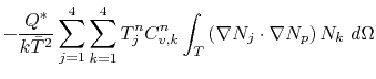
(4.46) is written as

$$\sum_{k=1}^{4} C_{v,k}^n M_{kp} - \sum_{k=1}^{4}C_{v,k}^{n-1} M_{... ...B\bar\T} \sum_{i=1}^4\sum_{k=1}^4 \symElecPot_i^n C_{v,k}^n \Theta_{ipk}\right.$$

$$\left. - \frac{\Q}{\kB\bar\T^2} \sum_{j=1}^4\sum_{k=1}^4 \T_j^n C... ...ar\T} \sum_{l=1}^4\sum_{k=1}^4 \symHydStress_l^n C_{v,k}^n \Theta_{lpk} \right]$$ (4.48)

$$+ \frac{\Delta t_n}{\symVacRelTime}\left( q\sum_{m=1}^4 C_{im,m}^n M_{mp} - \Ceq V_p\right) = 0,\qquad p=1,...,4.$$

In the above derivation the vacancy diffusivity is treated as a scalar diffusion coefficient. In order to take into account the anisotropy of diffusivity due to the mechanical stress, as presented in Section 3.2.2, a diffusivity tensor must be applied. This requires a slight modification of (4.48) to

$$\sum_{k=1}^{4} C_{v,k}^n M_{kp} - \sum_{k=1}^{4}C_{v,k}^{n-1} M_{... ...B\bar\T} \sum_{i=1}^4\sum_{k=1}^4 \symElecPot_i^n C_{v,k}^n \Theta_{ipk}\right.$$

$$\left. - \frac{\Q}{\kB\bar\T^2} \sum_{j=1}^4\sum_{k=1}^4 \T_j^n C... ...ar\T} \sum_{l=1}^4\sum_{k=1}^4 \symHydStress_l^n C_{v,k}^n \Theta_{lpk} \right]$$ (4.49)

$$+ \frac{\Delta t_n}{\symVacRelTime}\left( q\sum_{m=1}^4 C_{im,m}^n M_{mp} - \Ceq V_p\right) = 0,\qquad p=1,...,4.$$

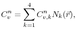
where the diffusivity tensor $\mathbf{D}$ is now incorporated into $K_{kp}$ and $\Theta_{ipk}$, given by

$$K_{ip} = \ensuremath{\int_{T}{\mathbf{D}\ensuremath{\nabla{{\symS... ...i}}}\ensuremath{\cdot}\ensuremath{\nabla{{\symShapeFun}_{p}}}}\ d{\symDomain}},$$ (4.50)

and

$$\Theta_{ipk} = \int_{T} \left(\mathbf{D}\ensuremath{\nabla{\symSh... ...h{\cdot}\ensuremath{\nabla{\symShapeFun_p}}\right) \symShapeFun_k\ d\symDomain.$$ (4.51)

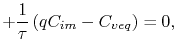
At material interfaces and grain boundaries the trapped vacancy concentration is governed by (3.76), rewritten here as

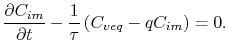
$$\ensuremath{\ensuremath{\frac{\partial \Cim}{\partial t}}} - \frac{1}{\symVacRelTime}\left(\Ceq-q\Cim\right) = 0.$$ (4.52)

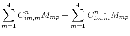
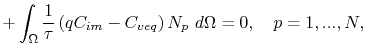
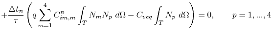
The finite element formulation of this equation follows the same procedure described above, which yields the discretization

$$\sum_{m=1}^{4} C_{im,m}^n M_{mp} - \sum_{m=1}^{4}C_{im,m}^{n-1} M_{mp}$$

$$+ q\frac{\Delta t_n}{\symVacRelTime}\sum_{m=1}^4 C_{im,m}^n M_{mp} - \frac{\Delta t_n}{\symVacRelTime}\Ceq V_p = 0,\qquad p=1,...,4.$$ (4.53)