, the modulus
  of the wave vector as a function of energy, the generalized density of
states
of the wave vector as a function of energy, the generalized density of
states  , and the scattering operator
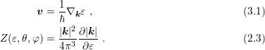
  . However, the velocity term
  and the
density of states
and the
density of states  are not independent and depend on the dispersion relation
  by
by
The SHE equations (2.34) and (2.35) incorporate material-specific properties by the velocity term
, the modulus of the wave vector as a function of energy, the generalized density of
states , and the scattering operator . However, the velocity term and the
density of states are not independent and depend on the dispersion relation
by
The second half of this chapter is devoted to the various scattering effects. Since scattering balances the energy gain of carriers due to the electric field, accurate expressions for the scattering operators are mandatory. Scattering mechanisms leading to a linear operator are discussed in Sec. 3.3, while the case of nonlinear scattering operators is investigated in Sec. 3.4.
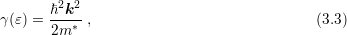
Due to the nonuniformity of the crystal lattice in silicon with respect to a change in direction, the dispersion relation linking the particle momentum with the particle energy cannot be accurately described by the idealized setting of an infinitely deep quantum well, for which the solution of Schrödinger’s equation yields a parabolic dependence of the energy on the wave vector:

 is the scaled Planck constant and
  is the effective mass. Still, this quadratic
relationship termed parabolic band approximation is a good approximation near the minimum of
the energy valley. Due to its simple analytical form, the parabolic dispersion relation is often
used up to high energies, for which it fails to provide an accurate description of the
material.
is the effective mass. Still, this quadratic
relationship termed parabolic band approximation is a good approximation near the minimum of
the energy valley. Due to its simple analytical form, the parabolic dispersion relation is often
used up to high energies, for which it fails to provide an accurate description of the
material.
A more accurate approximation to the band structure in silicon can be obtained by a slight modification of the form

 is called nonparabolicity factor; in the case
 one obtains again (3.2). More complicated analytical dependencies of the energy on the
wave vector are certainly possible, but (3.4) already provides very good results in the
low-energy regime. The choice
one obtains again (3.2). More complicated analytical dependencies of the energy on the
wave vector are certainly possible, but (3.4) already provides very good results in the
low-energy regime. The choice  provides a good approximation of the dispersion
relation for electrons in relaxed silicon. However, for kinetic energies above
provides a good approximation of the dispersion
relation for electrons in relaxed silicon. However, for kinetic energies above  eV the
nonparabolic approximation fails to describe the nonmonotonicity of the density of states in
silicon.
eV the
nonparabolic approximation fails to describe the nonmonotonicity of the density of states in
silicon.
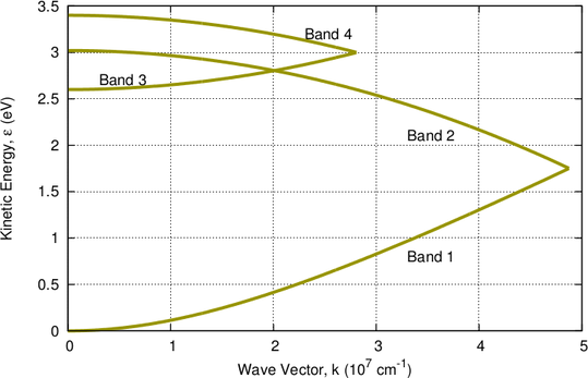
The deficiencies of the nonparabolic dispersion relation can be mitigated by a combination of four energy bands as proposed by Brunetti et. al. [11]:
 ,
,  and
and  respectively. The specific form of each
band is given by
respectively. The specific form of each
band is given by

 is computed from the individual
densities of states by a weighted sum:
is computed from the individual
densities of states by a weighted sum:

 ,
,  account for the number of equivalent
symmetrical bands of the
account for the number of equivalent
symmetrical bands of the  -th band can be found together with the other parameters of the
multi-band model in Tab. 3.1.
-th band can be found together with the other parameters of the
multi-band model in Tab. 3.1.
| Band |  |  |  |  |  |
| 1 | 0.320 | 0 | 1.75 | 6 | 0.35 |
| 2 | 0.712 | 1.75 | 3.02 | 6 | 0 |
| 3 | 0.750 | 2.60 | 3.00 | 12 | 0 |
| 4 | 0.750 | 3.00 | 3.40 | 12 | 0 |
 denotes the electron mass,
  the multiplicity of the respective band and
  is the
nonparabolicity factor. Each band extends from
is the
nonparabolicity factor. Each band extends from  to
to  .
. The BTE has in principle to be solved in each energy band with index  for a distribution
function
for a distribution
function  . However, since the individual distribution functions for each energy band are not
of particular interest, it is preferred to have a single dispersion relation describing the total
distribution function
. However, since the individual distribution functions for each energy band are not
of particular interest, it is preferred to have a single dispersion relation describing the total
distribution function  .
.
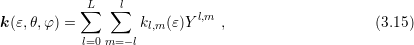
In order to account for the angular dependence of the energy on the wave vector in a semiconductor, the inverse dispersion relation is expanded as
 and nonnegative
  -values,
which are a multiple of four, lead to nonzero expansion coefficients. The expansion coefficients
-values,
which are a multiple of four, lead to nonzero expansion coefficients. The expansion coefficients
 can either be determined by an integration over spheres in
  -space, cf. (2.2), or by
minimization of certain target functionals such as the quadratic error of the scaled
moments
-space, cf. (2.2), or by
minimization of certain target functionals such as the quadratic error of the scaled
moments
 denotes the Brillouin zone.
A SHE of the valence band has been carried out by Kosina et al. [60] up to  eV.
Pham et al. [73] proposed a refined method for an expansion also including higher
energies. A fitted band structure based on SHE for the conduction band has been
presented by Matz et al. [69]. Due to the bijective mapping between energy and wave
vector, the velocity and the density of states are not in perfect agreement with full-band
data. Nevertheless, good results compared to the Monte Carlo method are obtained
[45].
eV.
Pham et al. [73] proposed a refined method for an expansion also including higher
energies. A fitted band structure based on SHE for the conduction band has been
presented by Matz et al. [69]. Due to the bijective mapping between energy and wave
vector, the velocity and the density of states are not in perfect agreement with full-band
data. Nevertheless, good results compared to the Monte Carlo method are obtained
[45].
 is labelled Modena model, as it is
also used in e.g. [42].
is labelled Modena model, as it is
also used in e.g. [42].
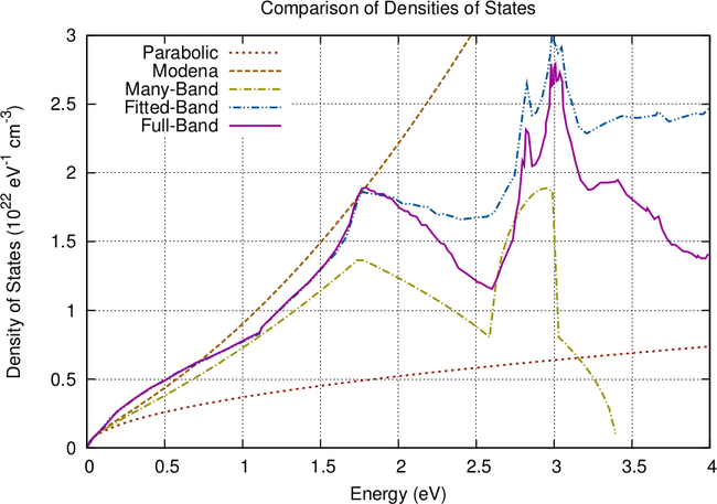
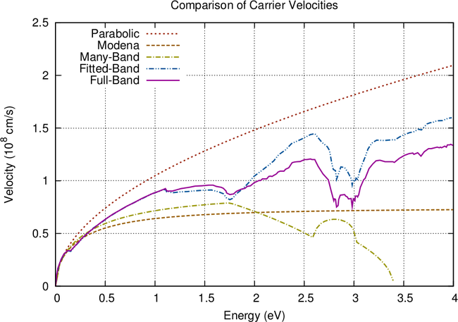
A comparison of the presented energy band models is given in Fig. 3.2. Slight deviations of
the many-band model and the full-band density of states are due to different Monte Carlo data
used in [11]. While the many-band model provides a good fit for the density of states, it fails to
approximate the carrier velocity and is worse than the nonparabolic model (3.3). As expected, the
fitted band model provides the best accuracy, even though approximations are less accurate at
energies above  eV.
eV.
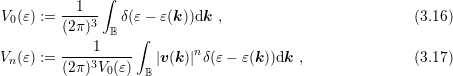
Vecchi et al. [107] used full-band Monte Carlo data for the velocity  and the generalized
density of states
and the generalized
density of states  for a first-order SHE. This is possible because in this case all terms with an
explicit representation of the band structure, i.e.
for a first-order SHE. This is possible because in this case all terms with an
explicit representation of the band structure, i.e.  , vanish. However, higher-order SHE does
not allow for a similar procedure, because the angular coupling term (2.33) does not
vanish any longer and an explicit expression for the modulus of the wave vector is
required.
, vanish. However, higher-order SHE does
not allow for a similar procedure, because the angular coupling term (2.33) does not
vanish any longer and an explicit expression for the modulus of the wave vector is
required.
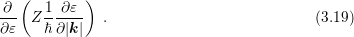
Recently, Jin et al. [48] suggested a reformulation as follows: Consider
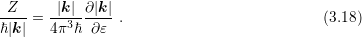
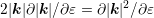 , the expression can be further rearranged
to
, the expression can be further rearranged
to

While the band structure links the particle energy with the particle momentum, it does not fully describe the propagation of carriers. In the presence of an electrostatic force, carriers would be accelerated and thus gain energy indefinitely unless scattering with the crystal lattice or with other carriers is included in the model. The most important scattering mechanisms are discussed in the following. The scattering operator is assumed to be given in the form

 ,
need to be taken into account when comparing scattering rates from different sources. Note that
the numerator of the prefactor differs from the numerator used for the spherical projection (2.6)
due to the assumption that scattering does not change spin. Moreover, it should be noted again
that the commonly written small sample volume
,
need to be taken into account when comparing scattering rates from different sources. Note that
the numerator of the prefactor differs from the numerator used for the spherical projection (2.6)
due to the assumption that scattering does not change spin. Moreover, it should be noted again
that the commonly written small sample volume  as prefactor for the scattering integral is not
written explicitly in the following.
as prefactor for the scattering integral is not
written explicitly in the following.
Atoms in the crystal lattice vibrate around their fixed equilibrium locations at nonzero
temperature. These vibrations are quantized by phonons with energy  . Acoustic
vibrations refer to a coherent movement of the lattice atoms out of their equilibrium positions.
Depending on the displacements with respect to the direction of propagation of the lattice wave,
transversal (TA) and longitudinal (LA) acoustic modes are distinguished.
. Acoustic
vibrations refer to a coherent movement of the lattice atoms out of their equilibrium positions.
Depending on the displacements with respect to the direction of propagation of the lattice wave,
transversal (TA) and longitudinal (LA) acoustic modes are distinguished.
Since the change in particle energy due to acoustic phonon scattering is very small, the process is typically modelled as an elastic process [47], which does not couple different energy levels. The scattering rate can thus be written as
 | (3.22) |
where the coefficient  is given by
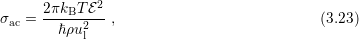
 is the deformation potential,
  is the density of mass, and
  is the longitudinal
sound velocity, cf. Tab. 3.2.
is the longitudinal
sound velocity, cf. Tab. 3.2.
| Si | Ge | |
 |  g/cm g/cm | 5.32 g/cm |
 |  cm/s cm/s |  cm/s cm/s |
 |  |  |
 |  eV eV |  eV eV |
 |  eV eV |  eV eV |
 and
and  are used to distinguish between electrons and holes.
Optical phonon scattering refers to an out-of-phase movement of lattice atoms. In ionic crystals, these vibrations can be excited by infrared radition, which explains the name. Similar to acoustic phonon scattering, transversal (TO) and longitudinal (LO) modes are distinguised.
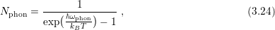
Since the involved phonon energies are rather high, cf. Tab. 3.3, optical phonon scattering is
typically modeled as an inelastic process leading to a change of the particle energy. With the
phonon occupation number  given by the Bose-Einstein statistics
 and the final state
  can be written as
![[
sop(x,k,k′) = σopNphon δ(ε(k) − ε(k′) + ℏωop)
+ (1+ N )δ(ε(k) − ε(k′) − ℏω )] ,
phon op](diss-et545x.png) | (3.25) |
where  is symmetric in
  and
and  and given by
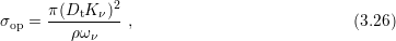
 , mass density
  , and phonon frequency
  . Values for the
individual modes can be found in Tab. 3.3. It should be noted that optical phonon
scattering couples the energy levels
. Values for the
individual modes can be found in Tab. 3.3. It should be noted that optical phonon
scattering couples the energy levels  ,
,  and
and  in an asymmetric
manner, because scattering from higher energy to lower energy is more likely than vice
versa.
in an asymmetric
manner, because scattering from higher energy to lower energy is more likely than vice
versa.
| Si | Ge | ||||
 | Mode |  |  |  |  |
 | TA |  eV/cm eV/cm |  meV meV |  eV/cm eV/cm |  meV meV |
 | LA |  eV/cm eV/cm |  meV meV |  eV/cm eV/cm |  meV meV |
 | LO |  eV/cm eV/cm |  meV meV |  eV/cm eV/cm |  meV meV |
 | TA |  eV/cm eV/cm |  meV meV |  eV/cm eV/cm |  meV meV |
 | LA |  eV/cm eV/cm |  meV meV |  eV/cm eV/cm |  meV meV |
 | TO |  eV/cm eV/cm |  meV meV |  eV/cm eV/cm |  meV meV |
Dopants in a semiconductor are fixed charges inside the crystal lattice. Since carriers are charged particles as well, their trajectories are influenced by these fixed charges, leading to a change of their momentum. The model by Brooks and Herring [10, 47] suggests an elastic scattering process with scattering coefficient

 is symmetric in
  and
and  and given by

 and
and  denote the acceptor
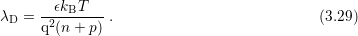
and donator concentrations respectively. The Debye length
denote the acceptor
and donator concentrations respectively. The Debye length  under assumption of local
equilibrium is given by
under assumption of local
equilibrium is given by
 . This complication can be circumvented by approximating the anisotropic
coefficient (3.27) by an elastic-isotropic process with the same momentum relaxation time
. This complication can be circumvented by approximating the anisotropic
coefficient (3.27) by an elastic-isotropic process with the same momentum relaxation time  [52]. The momentum relaxation time is computed for an isotropic dispersion relation by an
integration over the whole Brillouin zone and by weighting the change of direction of the
momentum [67]:
[52]. The momentum relaxation time is computed for an isotropic dispersion relation by an
integration over the whole Brillouin zone and by weighting the change of direction of the
momentum [67]:
 = =  ∫
Bsimp(x,k,k′)(1 − cos(θ))dk3 ∫
Bsimp(x,k,k′)(1 − cos(θ))dk3 |
 -axis for the integration in the Brillouin zone is chosen such that it is aligned with
 , hence the angle between
  and
and  is given by the inclination
  . Transformation to
spherical coordinates leads to
. Transformation to
spherical coordinates leads to
 = =  ∫
0∞∫
0π ∫
0∞∫
0π sinθdθZdε sinθdθZdε |
 is independent of the angles because of the assumption of an
isotropic dispersion relation. The integral over the inclination
is independent of the angles because of the assumption of an
isotropic dispersion relation. The integral over the inclination  can be computed analytically
as
can be computed analytically
as
∫
0π sinθdθ = sinθdθ =  ![[ 2 2 ]
ln(1 + 4λ2D|k|2)− --4λD-|k2|---
1 + 4λD|k|2](diss-et616x.png) . . |
![4 [ 2 2 ]
σimp;iso(x,k,k ′) = π-NIq---1--- ln(1 + 4λ2|k|2)− --4λD-|k-|-- (3.30)
ℏ ϵ2 4|k |4 D 1 + 4λ2D |k|2](diss-et617x.png)
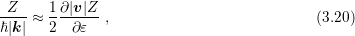
 should
be evaluated consistently with the approximated band, therefore the transformation (3.20) needs
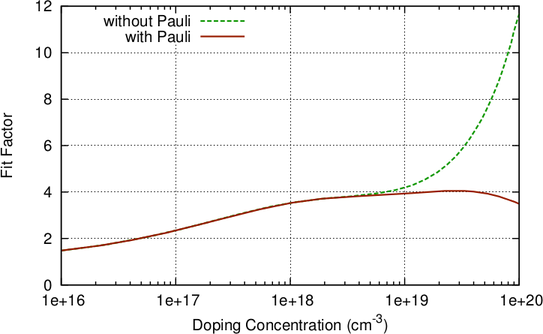
to be employed for the full-band case. Moreover, since the Brooks-Herring model fails to correctly
describe the carrier mobility at high doping concentrations, an empirical fit factor depicted in
Fig. 3.3 is usually employed additionally [52] in order to reproduce the Caughey-Thomas
expression for the mobility [15].
should
be evaluated consistently with the approximated band, therefore the transformation (3.20) needs
to be employed for the full-band case. Moreover, since the Brooks-Herring model fails to correctly
describe the carrier mobility at high doping concentrations, an empirical fit factor depicted in
Fig. 3.3 is usually employed additionally [52] in order to reproduce the Caughey-Thomas
expression for the mobility [15].
The scattering operator in low-density approximation for single carrier processes is linear, which is very attractive from a computational point of view. Consequently, scattering processes leading to a nonlinear scattering operator are often neglected in order to avoid nonlinear iteration schemes. In the following, two such types of scattering mechanisms are considered.
A high population of the conduction band can lead to the case that the distribution function
takes large values near the band edge, thus the term  cannot be approximated with
  any longer:
 | (3.31) |
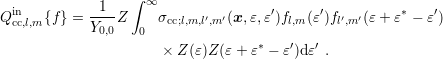
Repeating the steps from Sec. 2.2, one finally obtains for the projected in-scattering operator assuming velocity randomization and a scattering rate independent of the angles
![[ ][f] (x,ε± ℏω ,t)
Qiηn,l,m{f } = σ η(x, ε± ℏω η,ε) Zl,m(ε)− [f]l,m---0,0---------η---. (3.32)
Y0,0](diss-et623x.png)
![[ ]
Qout {f } = σ (x,ε,ε± ℏω )Z (ε± ℏω )− [f] (x, ε± ℏω ,t) [f]l,m . (3.33)
η,l,m η η 0,0 η 0,0 η Y0,0](diss-et624x.png)
Numerical results in [43] confirm that the low-density approximation does not have a high impact on macroscopic quantities such as the electron density or carrier velocities, but notable differences in the distribution function are obtained near the band edge. The carrier population is then shifted towards higher energies, because all states at lower energies are already populated.
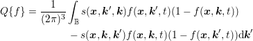
The linear scattering operators in Sec. 3.3 stem from the scattering of carriers with noncarriers. Very important for particularly the high energy tail of the distribution function is carrier-carrier scattering [79]. A carrier-carrier scattering mechanism requires that the two source states are occupied, and the two final states after scattering are empty. This leads to a scattering operator of the form
 | (3.34) |
where the scattering coefficient  now depends on the spatial location and on two pairs
of initial and final states. With a low-density approximation, the nonlinearity of degree four of the
carrier-carrier scattering operator reduces to second order:
now depends on the spatial location and on two pairs
of initial and final states. With a low-density approximation, the nonlinearity of degree four of the
carrier-carrier scattering operator reduces to second order:
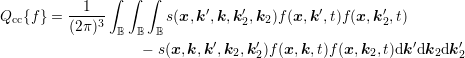 | (3.35) |
The scattering coefficient can be derived to be of the form [96, 99]


 replaced by the carrier density
  . Since
  only depends via
  on the difference of
the initial and the final state of one of the two carriers, the shorthand notation
on the difference of
the initial and the final state of one of the two carriers, the shorthand notation  is
used in the following.
is
used in the following.
Carrier-carrier scattering, particularly electron-electron scattering, has so far been discussed for first-order SHE only [108, 110]. In a joint work with Peter Willibald Lagger [62], the author has recently extended the method to arbitrary-order SHE, and the derivation is given in the following.
The scattering operator (3.35) is again split into an in-scattering term  and an
out-scattering term
and an
out-scattering term  as in Sec. 2.2. Inserting (3.36) into (3.35), one integration can be
carried out due to the momentum conservation. An integration with respect to
as in Sec. 2.2. Inserting (3.36) into (3.35), one integration can be
carried out due to the momentum conservation. An integration with respect to  yields

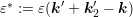 of the second particle involved in the
scattering process. A transformation of the two integrals to spherical coordinates leads
to
of the second particle involved in the
scattering process. A transformation of the two integrals to spherical coordinates leads
to
 | (3.39) |
where  and similarly for
  and
and  . A projection onto the spherical harmonic
 yields
 | (3.40) |
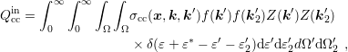
Up to now, no approximations have been applied. However, a direct evaluation of these nested integrals at each node in the simulation domain is certainly prohibitive for the use within a simulator due to excessive execution times. Consequently, the further derivation is based on the following two assumptions:
 can be taken as an external parameter. In principle, the energy
 of the second particle before scattering depends due to energy conservation on
all variables, i.e.
of the second particle before scattering depends due to energy conservation on
all variables, i.e.  . Because the asymptotically exponential
distribution of carriers with respect to energy, it is plausible, yet heuristic, that the
second particle has an energy close to the band gap. Since no additional information
about the second particle involved is known, the average energy is taken for
. Because the asymptotically exponential
distribution of carriers with respect to energy, it is plausible, yet heuristic, that the
second particle has an energy close to the band gap. Since no additional information
about the second particle involved is known, the average energy is taken for  ,
which is accessible due to the nonlinear iteration scheme required for the solution of
the discrete set of equations.
,
which is accessible due to the nonlinear iteration scheme required for the solution of
the discrete set of equations.
 can be expanded into spherical harmonics with
respect to
can be expanded into spherical harmonics with
respect to  and
and  . This can for example be achieved by using the isotropic
approximation (3.30) in order to obtain an isotropic scattering rate with equal
macroscopic relaxation time. As an alternative, one may directly compute a spherical
projection in order to obtain the expansion coefficients
. This can for example be achieved by using the isotropic
approximation (3.30) in order to obtain an isotropic scattering rate with equal
macroscopic relaxation time. As an alternative, one may directly compute a spherical
projection in order to obtain the expansion coefficients  of the
expansion
of the
expansion

 in the following. The same derivations
can also be carried out for the coefficients
in the following. The same derivations
can also be carried out for the coefficients  , but only the final result for this more
general case is given at the end of the derivation.
, but only the final result for this more
general case is given at the end of the derivation.With these assumptions, one can split the integrands to
 | (3.42) |
An expansion of  into spherical harmonics, the use of the delta distribution for an
elimination of the integral over
into spherical harmonics, the use of the delta distribution for an
elimination of the integral over  , and the assumption of spherical energy bands leads
to
, and the assumption of spherical energy bands leads
to
 | (3.43) |
Summing up, the projected in-scattering operator is given by
 | (3.44) |
For the more general case of an expansion of the scattering coefficient (3.41), one obtains again with the assumption of spherical energy bands
 | (3.45) |
The projection of the out-scattering operator starts with the same steps as for the in-scattering operator in order to arrive at
 | (3.46) |
The angles  and
and  depend in a complicated way on the other angles, therefore rather crude
simplifications are applied. Scattering with another carrier is to a first approximation determined
by the density of carriers at the particular location inside the device. Consequently, the
distribution function of the second particle, which is described by
depend in a complicated way on the other angles, therefore rather crude
simplifications are applied. Scattering with another carrier is to a first approximation determined
by the density of carriers at the particular location inside the device. Consequently, the
distribution function of the second particle, which is described by  and
and  , is
approximated by the isotropic part of the distribution function only, since it fully describes the
carrier density. With
, is
approximated by the isotropic part of the distribution function only, since it fully describes the
carrier density. With  and considering
  again as the
average energy, (3.46) simplifies to
again as the
average energy, (3.46) simplifies to
 | (3.47) |
The more general case of an expansion of the scattering coefficient (3.41) results in
 | (3.48) |
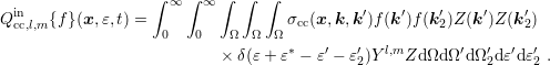
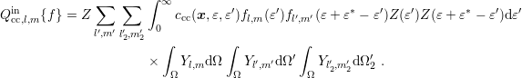
For the full projected scattering operator, one thus obtains
![Z ∫ ∞ [
Qcc,l,m {f} = --3- σcc(x,ε,ε′)f0,0(ε′)f0,0(ε+ ε∗ − ε′)
Y0,0 0 ]
− f0,0(ε∗)fl,m (ε)Z (ε)Z(ε+ ε∗ − ε′)dε′ .](diss-et672x.png) | (3.49) |
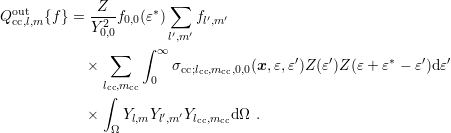
With the use of an expansion of the scattering coefficient (3.41), one obtains
![∑ ∑ ∫ ∞
Qcc,l,m {f} = -Z-- σcc;l ,m ,l′,m′ (x, ε,ε′)
Y02,0l ,m l′,m′ 0 cc cc cc cc
cc cccc cc [
Y0,0flcc,mcc(ε′)fl′cc,m′cc(ε + ε∗ − ε′)
∑ ∫ ]
− f0,0(ε∗) fl′,m′ Yl,mYl′,m ′Ylcc,mccdΩ
l′,m′ Ω
∗ ′ ′
× Z (ε)Z(ε+ ε − ε)dε .](diss-et673x.png) | (3.50) |
One can immediately see that the full scatter operator vanishes for the equilibrium case, where
 is given by a Maxwell distribution. Therefore, even though simplifications have been used for
the separate derivation of the projected equations for the in- and the out-scattering operators, the
resulting expressions are consistent.
is given by a Maxwell distribution. Therefore, even though simplifications have been used for
the separate derivation of the projected equations for the in- and the out-scattering operators, the
resulting expressions are consistent.