Chapter 4
Structural Properties
The SHE equations furnish a number of interesting structural properties, which are the topic
of this chapter. All properties are discussed on the continuous level and result from
certain symmetries of the underlying physical processes. Consequently, no additional
assumptions about a particular discretization method need to be imposed and the same
structural properties hold true for the system of discretized linear equations as outlined in
Chap. 5.
In Sec. 4.1 the coupling between the SHE equations is investigated and a scheme for the
lossless compression of the system matrix is proposed, which greatly reduces the memory
consumption of the SHE method at high expansion orders. The different boundary
conditions used for the SHE method are discussed in Sec. 4.4 and extensions to the system
matrix compression scheme are proposed in order to handle them. This chapter closes
with some numerical results demonstrating the benefits of the proposed compression
scheme.
4.1 Sparse Coupling for Spherical Energy Bands
As already noted in Sec. 2.3, the terms ![′ ′
[Y l,m ]l,m](diss-et675x.png) ,
,  and
and  determine the coupling
among the projected equations (2.30). If all coupling coefficients were multiples of the Kronecker
delta, then the SHE equations were decoupled and could be solved individually. On the contrary,
if all coupling coefficients were nonzero, all projected equations were coupled with each
other. In analogy to systems of linear equations described by matrices, one is typically
interested in a weak coupling, which typically accelerates the solution process, and
on the other hand leads to lower memory requirements. A closer inspection of the
coupling structure for spherically symmetric dispersion relations is carried out in this
section.
determine the coupling
among the projected equations (2.30). If all coupling coefficients were multiples of the Kronecker
delta, then the SHE equations were decoupled and could be solved individually. On the contrary,
if all coupling coefficients were nonzero, all projected equations were coupled with each
other. In analogy to systems of linear equations described by matrices, one is typically
interested in a weak coupling, which typically accelerates the solution process, and
on the other hand leads to lower memory requirements. A closer inspection of the
coupling structure for spherically symmetric dispersion relations is carried out in this
section.
For general band structures, the symmetry of the underlying processes leads to the following
result: [53]
Theorem 1 (Jungemann et. al.). For a spherical harmonics expansion up to order
 with
with  , there holds for all
  ,
,  and
and
| j2i,m2i′,m′
= j2i+1,m2i′+1,m′
= 0, Γ2i,m2i′,m′
= Γ2i+1,m2i′+1,m′
= 0 . | | |
The essence of this theorem is that all nonzero coupling coefficients possess different
parities in the leading indices. This small structural information about the coupling was
already used for a preprocessing step for the solution of the discretized equations in
[53].
Under the assumption of spherical energy bands, i.e.  , the velocity
  , the
modulus of the wave vector
, the
modulus of the wave vector  and the generalized density of states only depend on the energy
 , but not on the angles
  . Consequently, (2.31), (2.32) and (2.31) are rewritten
as
. Consequently, (2.31), (2.32) and (2.31) are rewritten
as
![l′,m ′ l′,m ′
[Y ]l,m = δl,m∫ , (4.1)
l′,m ′ l′,m ′
jl,m = vZ Yl,meεYl′,m′dΩ =: vZa l,m , (4.2)
′ ′ Z ∫ ( ∂Y 1 ∂Y ) Z ′ ′
Γ ll,,mm = ---- --l,m-eθ + -------l,me φ Yl′,m′dΩ =: ----bll,,mm , (4.3)
ℏ|k| ∂ θ sin θ ∂ φ ℏ|k|](diss-et688x.png) where
where  denotes the Kronecker delta and
  . A similar decomposition is possible with
the full-band modification (3.20).
. A similar decomposition is possible with
the full-band modification (3.20).
The coupling between index pairs  and
and  is determined by the integral terms
 and
and  only. As shown by the author, it turns out that the coupling is rather
weak:
only. As shown by the author, it turns out that the coupling is rather
weak:
A rather lengthy and technical proof is given in [87] and makes use of recurrence relations
and orthogonalities of trigonometric functions and associated Legendre functions.
Thm. 2 is very important for large expansion orders  : The total number of unknown
expansion coefficients is
: The total number of unknown
expansion coefficients is  , but according to the result of the theorem, each
  is
directly coupled with at most ten other coefficients. It should also be noted that the weak
coupling stated in Thm. 2 has already been observed for less general situations in earlier
publications [78, 37].
is
directly coupled with at most ten other coefficients. It should also be noted that the weak
coupling stated in Thm. 2 has already been observed for less general situations in earlier
publications [78, 37].
Next, the structure of the SHE equations (2.30) for spherical energy bands is investigated in
depth. Unlike the presentation in [87], the structure is investigated already at the
continuous level, which has the advantage of covering a wider class of discretization
schemes and less notational clutter. Due to the equivalence of (2.30) and (2.38) for
spherical energy bands, the results in this section apply equally to an expansion of the
distribution function  and to an expansion of the generalized distribution function
 .
.
A motivation for a first-order expansion is now given, then the scheme is extended to general
expansion orders. Ignoring the stabilization using MEDS in a first step, the four SHE equations
using Einstein summation convention read
 + vZa0,0l′,m′
⋅∇xfl′,m′ + + vZa0,0l′,m′
⋅∇xfl′,m′ +  b0,0l′,m′
⋅F + ∑
η b0,0l′,m′
⋅F + ∑
η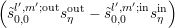 fl′,m′ fl′,m′ | = 0 , | |
|
 + vZa1,−1l′,m′
⋅∇xfl′,m′ + + vZa1,−1l′,m′
⋅∇xfl′,m′ +  b1,−1l′,m′
⋅F + ∑
η b1,−1l′,m′
⋅F + ∑
η fl′,m′ fl′,m′ | = 0 , | |
|
 + vZa1,0l′,m′
⋅∇xfl′,m′ + + vZa1,0l′,m′
⋅∇xfl′,m′ +  b1,0l′,m′
⋅F + ∑
η b1,0l′,m′
⋅F + ∑
η fl′,m′ fl′,m′ | = 0 , | |
|
 + vZa1,1l′,m′
⋅∇xfl′,m′ + + vZa1,1l′,m′
⋅∇xfl′,m′ +  b1,1l′,m′
⋅F + ∑
η b1,1l′,m′
⋅F + ∑
η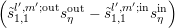 fl′,m′ fl′,m′ | = 0 . | | |
The terms  and
and  may be operators in order to take shifts of the
arguments of the distribution function into account and denote the angular coupling of the
scattering operator and reduce to Kronecker deltas when scattering processes are modeled as
velocity randomizing, cf. Sec. 2.2.
may be operators in order to take shifts of the
arguments of the distribution function into account and denote the angular coupling of the
scattering operator and reduce to Kronecker deltas when scattering processes are modeled as
velocity randomizing, cf. Sec. 2.2.
This continuous linear system of partial differential equations can be written in operator
matrix form as
 | (4.4) |
where the gradient and the time derivative act as an operator on the expansion coefficients, not
on the coefficient matrices. The crucial observation now is that all entries in each of the matrices
are independent of the spatial variable  as well as of total energy
  . Writing
  and
and  in components,
F(x) =  ,x = ,x =  , , | | |
the considered first-order system can thus be written as
 where the matrices
  ,
,  ,
,  ,
,  and
and  are given by the respective matrices in
(4.4).
are given by the respective matrices in
(4.4).
For the case of a general expansion order  , an enumeration of the index pairs
  is
required. Let
is
required. Let  denote such a mapping, for instance
  . Repeating the
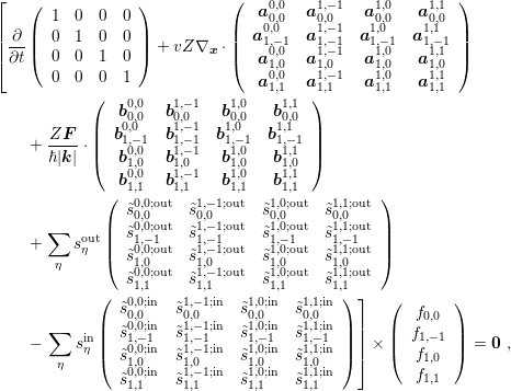
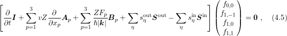
calculation for the general case, one obtains that the operator matrix
. Repeating the
calculation for the general case, one obtains that the operator matrix  for the SHE equations
can be written as
for the SHE equations
can be written as
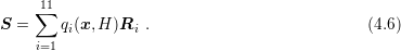 The
spatial terms
The
spatial terms  are given by
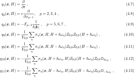 with
the energy shift operator
with
the energy shift operator  . Note that some of the terms
  evaluate to zero if one- or two-dimensional simulations are carried out. The angular coupling
matrices
evaluate to zero if one- or two-dimensional simulations are carried out. The angular coupling
matrices  are determined by
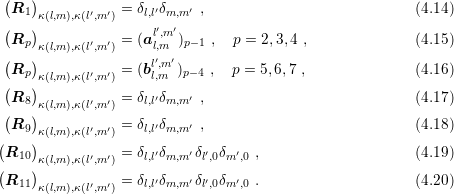 Hence, the full continuous system of equations
  can be composed out of continuous
spatial terms
can be composed out of continuous
spatial terms  and constant angular coupling matrices
  ,
,  . It is
worthwhile to mention that each of the coefficient pair
. It is
worthwhile to mention that each of the coefficient pair  can be replaced by a
single coefficient, and similarly for
can be replaced by a
single coefficient, and similarly for  if only elastic scattering is considered. In
analogy, each of the pairs
if only elastic scattering is considered. In
analogy, each of the pairs  and
and  can be replaced by a single matrix
[87].
can be replaced by a single matrix
[87].
The decomposition of the continuous case is preserved after spatial discretization. To see
this, let  denote the matrices arising from an arbitrary discretization of
the terms
denote the matrices arising from an arbitrary discretization of
the terms  . In most cases, a finite volume or a finite element method will
be employed, but also less widespread techniques such as wavelet methods could be
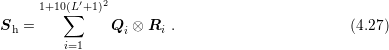
used. Then, the discrete system matrix
. In most cases, a finite volume or a finite element method will
be employed, but also less widespread techniques such as wavelet methods could be
used. Then, the discrete system matrix  for the SHE equations can be written
as
for the SHE equations can be written
as
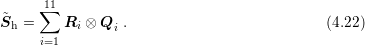
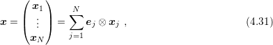
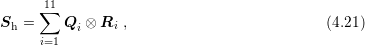 where
where  denotes the Kronecker product (cf. A.1 for the definition). After a suitable
rearrangement of unknowns, the system matrix could also be written in the equivalent
form
denotes the Kronecker product (cf. A.1 for the definition). After a suitable
rearrangement of unknowns, the system matrix could also be written in the equivalent
form
 The
advantage of a representation using sums of Kronecker products is the considerably smaller
memory required for the factors. For a SHE of order
The
advantage of a representation using sums of Kronecker products is the considerably smaller
memory required for the factors. For a SHE of order  , the matrices
  are of size
 and sparse according to Sec. 4.1. For a spatial discretization using
  unknowns, the matrices
  are of dimension
  and typically sparse, hence the full system
matrix
and typically sparse, hence the full system
matrix  is of dimension
  . While the explicit storage of a sparse
system
. While the explicit storage of a sparse
system  thus requires
  memory, a storage of the Kronecker product
factors requires
memory, a storage of the Kronecker product
factors requires  memory only, which is a considerable difference already for
  or
or  .
.
In light of the memory requirements for the system matrix it is also worthwhile to
point out the importance of Thm. 2: Without the sparsity of coupling coefficients and
without the use of a Kronecker representation,  memory is
required. With the sparsity of coupling coefficients, only
memory is
required. With the sparsity of coupling coefficients, only  memory is required for
a full representation of
memory is required for
a full representation of  , which is further reduced to
  when using a
Kronecker product representation. Since typical values of
when using a
Kronecker product representation. Since typical values of  are in the range three
to seven, the memory savings due to Thm. 2 combined with (4.21) can be orders of
magnitude.
are in the range three
to seven, the memory savings due to Thm. 2 combined with (4.21) can be orders of
magnitude.
4.2 Coupling for Nonspherical Energy Bands
The matrix compression described in the previous section relies on the factorizations (4.2) and
(4.3) of the coupling terms  and
and  , such that the factors depend on either energy (and
possibly the spatial location) or on the indices
, such that the factors depend on either energy (and
possibly the spatial location) or on the indices  ,
,  ,
,  and
and  , but not on both. Moreover,
the derivation requires that the density of states does not show an angular dependence. However,
in the case of nonspherical energy bands, these three terms depend on energy and on
angles.
, but not on both. Moreover,
the derivation requires that the density of states does not show an angular dependence. However,
in the case of nonspherical energy bands, these three terms depend on energy and on
angles.
In order to decouple the radial (energy) contributions from the angular ones for nonspherical
energy band models, a spherical projection up to order  of the coupling terms can be
performed by approximating [53]
of the coupling terms can be
performed by approximating [53]
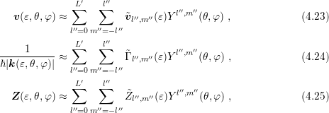 where the expansion coefficients are given for
  by
by
 l′′,m′′(ε) l′′,m′′(ε) | = ∫
Ωv(ε,θ,φ)Y l′′,m′′
(θ,φ)dΩ , | |
|
 l′′,m′′(ε) l′′,m′′(ε) | = ∫
Ω Y l′′,m′′
(θ,φ)dΩ , Y l′′,m′′
(θ,φ)dΩ , | |
|
 l′′,m′′(ε) l′′,m′′(ε) | = ∫
ΩZ(ε,θ,φ)Y l′′,m′′
(θ,φ)dΩ . | | |
For simplicity, the expansion order  , which depends on the complexity of the band structure,
is taken to be the same for
, which depends on the complexity of the band structure,
is taken to be the same for  ,
,  and
and  . In a slightly different context, values of
 have been used in [73] and [69] for an expansion of
  , and good accuracy has been
obtained. On the other hand, a spherically symmetric velocity profile is exactly recovered by an
expansion order
, and good accuracy has been
obtained. On the other hand, a spherically symmetric velocity profile is exactly recovered by an
expansion order  .
.
The expansion order of the generalized density of states  is implicitly coupled to the
expansion order
is implicitly coupled to the
expansion order  of the distribution function by the scattering operator (2.23). Thus, even if
 is expanded up to order
  , only expansion terms up to order
  can be considered. For
this reason
can be considered. For
this reason  is assumed in the following.
Substitution of the expansions (4.23) and (4.24) into (4.2) and (4.3) yields
| jl,ml′,m′
| =  l′′,m′′(ε)∫
ΩY l,mY l′,m′
Y l′′,m′′
dΩ =: vl′′,m′′(ε)al,ml′,m′;l′′,m′′
, l′′,m′′(ε)∫
ΩY l,mY l′,m′
Y l′′,m′′
dΩ =: vl′′,m′′(ε)al,ml′,m′;l′′,m′′
, | |
|
| Γl,ml′,m′
| =  l′′,m′′(ε)∫
Ω l′′,m′′(ε)∫
Ω  eθ + eθ +   eφ eφ Y l′,m′
Y l′′,m′′
dΩ =: Γl′′,m′′(ε)bl,ml′,m′;l′′,m′′
, Y l′,m′
Y l′′,m′′
dΩ =: Γl′′,m′′(ε)bl,ml′,m′;l′′,m′′
, | | |
so that in both cases a sum of  decoupled terms is obtained. Note that in the case of
spherical energy bands, the sum degenerates to a single term. Repeating the steps from the
previous section, the continuous system of partial differential equations
decoupled terms is obtained. Note that in the case of
spherical energy bands, the sum degenerates to a single term. Repeating the steps from the
previous section, the continuous system of partial differential equations  can be written similar
to (4.6) in the form
can be written similar
to (4.6) in the form
 while
the discrete system matrix
while
the discrete system matrix  can be written in analogy to (4.21) as
 The
entries of the coupling matrices due to
The
entries of the coupling matrices due to  are directly obtained from the Wigner
3jm-symbols, cf. A.2. The sparsity of the coupling matrices due to
are directly obtained from the Wigner
3jm-symbols, cf. A.2. The sparsity of the coupling matrices due to  is not clear at
present, but a similar structure is expected. Assuming for simplicity dense spherical harmonics
coupling matrices, the system matrix can be stored using at most
is not clear at
present, but a similar structure is expected. Assuming for simplicity dense spherical harmonics
coupling matrices, the system matrix can be stored using at most  memory,
where in typical situations
memory,
where in typical situations  .
.
4.3 Stabilization Schemes
The stabilization schemes discussed in Sec. 2.3 lead to different equations for even-order and
odd-order projected equations. Since MEDS basically exchanges the summation index and the
sign of the coupling term  , the representations (4.6) and (4.26) can extended
to
, the representations (4.6) and (4.26) can extended
to
 where
where  denotes the number of matrices.
  refers to the even-order equations and is obtained
from
refers to the even-order equations and is obtained
from  by setting all rows
  to zero.
  is obtained from
  by transposition
and zeroing all rows
by transposition
and zeroing all rows  of the transposed matrix. In addition, signs are swapped in terms
affected by MEDS.
of the transposed matrix. In addition, signs are swapped in terms
affected by MEDS.
For the discretization it is assumed that even-order harmonics can be discretized in a different
manner than odd-order harmonics. If all even-order unknowns are enumerated first, the system
matrix  has a block-structure of the form
 The
even-to-even coupling matrix
The
even-to-even coupling matrix  and the odd-to-odd coupling matrix
  are square matrices
and determined according to Thm. 1 or Thm. 2 only by the projected time derivative
are square matrices
and determined according to Thm. 1 or Thm. 2 only by the projected time derivative
![∂[f]l,m∕∂t](diss-et835x.png) and the projected scattering operator
and the projected scattering operator  . The even-to-odd coupling matrix
 is not necessarily square and determined by the free-streaming operator with sparsity
pattern given by Thm. 2. The odd-to-even coupling matrix
is not necessarily square and determined by the free-streaming operator with sparsity
pattern given by Thm. 2. The odd-to-even coupling matrix  is rectangular in general and
determined by the free-streaming operator and for nonspherical bands also by the scattering
operator
is rectangular in general and
determined by the free-streaming operator and for nonspherical bands also by the scattering
operator  , cf. (2.23).
Since the coupling structure of the scattering operator is explicitly given by (2.23), the
structure of  and
and  is as follows:
Theorem 3. The following statements hold true for a system matrix (4.29) obtained from a
discretization of the stabilized SHE equations in steady-state with velocity-randomizing scattering
processes only:
- The matrix
 is diagonal.
- For spherical energy bands without considering inelastic scattering,
 is diagonal.
This structural information is very important for the construction of solution schemes in
Sec. 4.5.
4.4 Boundary Conditions
Only the discretization of the resulting system of partial differential equations in the interior of
the simulation domain has been considered in an abstract fashion so far. At the boundary,
suitable conditions need to be imposed and incorporated into the proposed compression
scheme.
At all noncontact boundaries, homogeneous Neumann boundary conditions are imposed
[78, 53, 42], which can be directly included in the proposed compression scheme, because no
additional boundary terms appear. At the contact boundaries, two different types of boundary
conditions are typically imposed. The first type are Dirichlet boundary conditions [78], where
the distribution function is set to a Maxwell distribution. Hence, the expansion coefficient  is
set according to (2.1), while
is
set according to (2.1), while  is set to zero for
  . This it either enforced by
replacing the corresponding matrix row with unity in the diagonal and zeros elsewhere as well as
setting the appropriate value at the right hand side vector, or by directly absorbing the
known values to the load vector. For the proposed compression scheme, the second
way is of advantage, because in that case boundary conditions do not alter the matrix
structure.
. This it either enforced by
replacing the corresponding matrix row with unity in the diagonal and zeros elsewhere as well as
setting the appropriate value at the right hand side vector, or by directly absorbing the
known values to the load vector. For the proposed compression scheme, the second
way is of advantage, because in that case boundary conditions do not alter the matrix
structure.
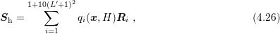
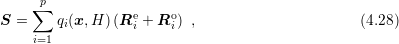
The second type of contact boundary conditions is a Robin-type generation/recombination
process [53]
γl,m(ε) = − , , | | |
where  denotes the equilibrium Maxwell distribution, or, similar in structure, a surface
generation process of the form [42]
denotes the equilibrium Maxwell distribution, or, similar in structure, a surface
generation process of the form [42]
| Γs = [feq(k′)ϑ(v ⋅n) + f(k′)ϑ(−v ⋅n)]v ⋅n , | | |
where  denotes the step function and
  is the unit surface normal vector pointing into the
device. This type of boundary conditions leads to additional entries in the system matrix due to
the surface boundary integrals. Consequently, the scheme needs to be adjusted and written in the
form
is the unit surface normal vector pointing into the
device. This type of boundary conditions leads to additional entries in the system matrix due to
the surface boundary integrals. Consequently, the scheme needs to be adjusted and written in the
form
 where
where  contains the discretized equations for all interior points as given by (4.21), (4.27) or
(4.29), and
contains the discretized equations for all interior points as given by (4.21), (4.27) or
(4.29), and  consists of the discretized contact boundary terms. Since the number of
contact boundary points is much smaller than the total number of grid points
consists of the discretized contact boundary terms. Since the number of
contact boundary points is much smaller than the total number of grid points  , the sparse
matrix
, the sparse
matrix  can be set up without compression scheme and the additional memory
requirements are negligible.
can be set up without compression scheme and the additional memory
requirements are negligible.
As can be easily verified,  can also be written as a sum of Kronecker products.
Consequently, the following discussions are based on the case of Dirichlet boundary conditions,
but are also applicable to the more general case including Robin-type boundary conditions, which
only add additional summands.
can also be written as a sum of Kronecker products.
Consequently, the following discussions are based on the case of Dirichlet boundary conditions,
but are also applicable to the more general case including Robin-type boundary conditions, which
only add additional summands.
4.5 Solution of the Linear System
The system matrix representation introduced in the previous sections is of use only if the
resulting scheme can be solved without recovering the full matrix again. Such a reconstruction is,
in principle, necessary if direct solvers such as the Gauss algorithm are used, because the matrix
structure is altered in a way that destroys the block structure. In contrast, for many popular
iterative solvers from the family of Krylov methods, it is usually sufficient to provide
matrix-vector multiplications. Therefore, methods to compute the matrix-vector product  for a given vector
  are discuss first.
Given a system matrix of the form (4.21) or (4.27), it is well known that a row-by-row
reconstruction of the compressed matrix  for the matrix-vector product is not
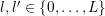
efficient. Therefore, the vector
for the matrix-vector product is not
efficient. Therefore, the vector  is decomposed into
  blocks of size
  by
by
 where
where  is the
  -th column vector of the identity matrix. The matrix-vector product can now
be written as
-th column vector of the identity matrix. The matrix-vector product can now
be written as
![p N
[∑ ][∑ ]
Sx = Qi ⊗ Ri ej ⊗ xj (4.32)
i=1 j=1
∑p ∑N
= (Qiej) ⊗ (Rixj) . (4.33)
i=1j=1](diss-et866x.png) Here,
the product
Here,
the product  is simply the
  -th column of
  .
.
In the case of spherical energy bands, it can be shown that the matrix-vector multiplication
requires slightly less computational effort than the uncompressed case [87]. As discussed in
Sec. 4.2, nonspherical bands lead to a larger number of summands, thus leading to a higher
computational effort for the matrix-vector multiplications compared to the uncompressed case.
Nevertheless, the additional computational effort is increased only moderately, while the memory
requirements can be reduced significantly.
Recent publications report the elimination of odd order unknowns in a preprocessing step
[53, 42]. Moreover, it has been shown that for a first-order expansion the system matrix after
elimination of odd order unknowns is an  -matrix [42]. Furthermore, numerical experiments
indicate a considerable improvement in the convergence of iterative solvers. However, for a matrix
structure as given by (4.29), a direct elimination of odd order unknowns would destroy the
representation of the system matrix
-matrix [42]. Furthermore, numerical experiments
indicate a considerable improvement in the convergence of iterative solvers. However, for a matrix
structure as given by (4.29), a direct elimination of odd order unknowns would destroy the
representation of the system matrix  as a sum of Kronecker products. Writing the system
as
as a sum of Kronecker products. Writing the system
as
 with
the vector of unknowns
with
the vector of unknowns  split into
  and
and  as unknowns associated with even and odd
order harmonics respectively and analogously for the right hand side vector
as unknowns associated with even and odd
order harmonics respectively and analogously for the right hand side vector  , the elimination of
odd order unknowns is carried out using the Schur complement:
, the elimination of
odd order unknowns is carried out using the Schur complement:
 According to Thm. 3,
  is a diagonal matrix, thus the inverse is directly available. The other
matrix-vector products are carried out as discussed in the beginning of this section. Note that the
matrix
is a diagonal matrix, thus the inverse is directly available. The other
matrix-vector products are carried out as discussed in the beginning of this section. Note that the
matrix 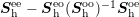 is never set up explicitly.
In contrast to a matrix-vector multiplication with the full system matrix  , where the
proposed matrix compression scheme requires approximately the same computational effort, a
matrix-vector multiplication with the condensed matrix
, where the
proposed matrix compression scheme requires approximately the same computational effort, a
matrix-vector multiplication with the condensed matrix  is more
expensive than a matrix-vector multiplication with a fully set up condensed matrix. The penalty
is quantified in Sec. 4.6.
is more
expensive than a matrix-vector multiplication with a fully set up condensed matrix. The penalty
is quantified in Sec. 4.6.
With a system matrix representation of the form (4.21), the total memory needed for the SHE
equations is essentially given by the memory required for the unknowns, which adds another
perspective on the selection of the iterative solver. Since  , the system matrix
  is not symmetric. Moreover, numerical experiments indicate that the matrix
  is
indefinite, thus many popular solvers cannot be used. A popular solver for indefinite
problems is GMRES [89, 112], which is typically restarted after, say,
is
indefinite, thus many popular solvers cannot be used. A popular solver for indefinite
problems is GMRES [89, 112], which is typically restarted after, say,  steps and
denoted by GMRES(
steps and
denoted by GMRES( ). Since GMRES has been used in recent publications on SHE
simulations [53, 42], it deserves a closer inspection. For a system with
). Since GMRES has been used in recent publications on SHE
simulations [53, 42], it deserves a closer inspection. For a system with  unknowns, the
memory required by GMRES(
unknowns, the
memory required by GMRES( ) during the solution process is
  . In typical
applications, in which the system matrix is uncompressed, this additional memory
approximately equals the amount of memory needed for the storage of the system
matrix, hence it is not a major concern. However, with the system matrix representation
(4.6) the memory needed for the unknowns is dominant, thus the additional memory
for GMRES(
. In typical
applications, in which the system matrix is uncompressed, this additional memory
approximately equals the amount of memory needed for the storage of the system
matrix, hence it is not a major concern. However, with the system matrix representation
(4.6) the memory needed for the unknowns is dominant, thus the additional memory
for GMRES( ) directly pushes the overall memory requirements from
  to
to
 . The number of steps
  is typically chosen between
  and
and  as smaller
values may lead to smaller convergence rates or the solver may even fail to converge
within a reasonable number of iterations. Hence, it is concluded that GMRES(
as smaller
values may lead to smaller convergence rates or the solver may even fail to converge
within a reasonable number of iterations. Hence, it is concluded that GMRES( )
is too expensive for SHE simulations when using the representation (4.6). Instead,
iterative solvers with smaller memory consumption such as BiCGStab [102] should be
used.
)
is too expensive for SHE simulations when using the representation (4.6). Instead,
iterative solvers with smaller memory consumption such as BiCGStab [102] should be
used.
4.6 Results
In this section execution times and memory requirements of the Kronecker product representation
(4.6) using a single core of a machine with a Core 2 Quad 9550 CPU are reported. To simplify
wording, the representation (4.6) will be referred to as matrix compression scheme. All
simulations were carried out for a stationary two-dimensional device on a regular staggered grid
with  nodes in
  -space for various expansion orders. Spherical energy
bands were assumed and the
-space for various expansion orders. Spherical energy
bands were assumed and the  -transform and MEDS were used for stabilization. A
fixed potential distribution was applied to the device to obtain comparable results.
For self-consistency with the Poisson equation using a Newton scheme, similar results
can in principle be obtained by application of the matrix compression scheme to the
Jacobian.
-transform and MEDS were used for stabilization. A
fixed potential distribution was applied to the device to obtain comparable results.
For self-consistency with the Poisson equation using a Newton scheme, similar results
can in principle be obtained by application of the matrix compression scheme to the
Jacobian.
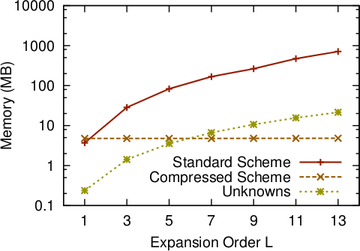
First, memory requirements for the storage of the system matrix are compared. The total
number of entries stored in the matrix were extracted, multiplied by three to account for row and
column indices. Eight bytes per entry for double precision are used. In this way, the influence of
different sparse matrix storage schemes is eliminated. The results in Fig. 4.1 and Fig. 4.2
clearly demonstrate the asymptotic advantage of (4.6): While no savings are observed
at  , memory savings of a factor of
  are obtained already at an expansion
order of
are obtained already at an expansion
order of  . At
. At  , this factor grows to
  . In particular, the memory
requirement for the matrix compression scheme shows only a weak dependence on
. In particular, the memory
requirement for the matrix compression scheme shows only a weak dependence on  and is determined only by the additional memory needed for the coupling matrices
 in (4.14)-(4.20). With increasing expansion order
  , the additional memory
requirements for the compressed scheme grow quadratically with
, the additional memory
requirements for the compressed scheme grow quadratically with  because of the
  spherical harmonics of degree smaller or equal to
  . Even at
  the additional
memory compared to
the additional
memory compared to  is less than one megabyte. Consequently, the memory
used for the unknowns dominates already at moderate values of
is less than one megabyte. Consequently, the memory
used for the unknowns dominates already at moderate values of  , cf. Fig. 4.1 and
Fig. 4.2.
, cf. Fig. 4.1 and
Fig. 4.2.
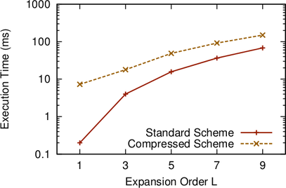
Execution times for matrix-vector multiplications are compared in Fig. 4.3 for the case of a
full system matrix and the system matrix with odd expansion orders eliminated. For the lowest
expansion order  , the matrix compression does not pay off and execution times are by a
factor of two larger then for the standard storage scheme. This is due to the additional structural
overhead of the compressed scheme at expansion order
, the matrix compression does not pay off and execution times are by a
factor of two larger then for the standard storage scheme. This is due to the additional structural
overhead of the compressed scheme at expansion order  , where no compression effect
occurs. However, for larger values of
, where no compression effect
occurs. However, for larger values of  , the matrix compression scheme leads to faster
matrix-vector multiplications with the full system of linear equations. An additional performance
gain of about ten percent is observed. Comparing execution times for the condensed
system, where odd order unknowns have been eliminated in a preprocessing step, the
runtime penalty for matrix-vector multiplication is a factor of
, the matrix compression scheme leads to faster
matrix-vector multiplications with the full system of linear equations. An additional performance
gain of about ten percent is observed. Comparing execution times for the condensed
system, where odd order unknowns have been eliminated in a preprocessing step, the
runtime penalty for matrix-vector multiplication is a factor of  at
at  , but in
this case there is no compression effect anyway. At
, but in
this case there is no compression effect anyway. At  , the runtime penalty is
only a factor of three and drops to slightly above two at
, the runtime penalty is
only a factor of three and drops to slightly above two at  . In conclusion, the
matrix compression scheme allows for a trade-off between memory consumption and
execution time, where the memory reduction is much larger than the penalty on execution
times.
. In conclusion, the
matrix compression scheme allows for a trade-off between memory consumption and
execution time, where the memory reduction is much larger than the penalty on execution
times.
|
|
|
|
|
|
| L | GMRES(50) | GMRES(30) | GMRES(10) | BiCGStab | Unknowns |
|
|
|
|
|
|
| 1 | 10.2 MB | 6.2 MB | 2.2 MB | 1.2 MB | 0.2 MB |
| 3 | 71.4 MB | 43.4 MB | 15.4 MB | 8.4 MB | 1.4 MB |
| 5 | 178.5 MB | 108.5 MB | 38.5 MB | 21.0 MB | 3.5 MB |
| 7 | 336.6 MB | 204.7 MB | 72.6 MB | 39.6 MB | 6.6 MB |
| 9 | 545.7 MB | 331.7 MB | 117.7 MB | 64.2 MB | 10.7 MB |
| 11 | 800.7 MB | 486.7 MB | 172.7 MB | 93.5 MB | 15.7 MB |
| 13 | 1101.6 MB | 669.6 MB | 237.6 MB | 129.6 MB | 21.6 MB |
|
|
|
|
|
|
| |
Table 4.1: Additional memory requirements of the linear solvers GMRES(s) with different
values of  and BiCGStab compared to the memory needed for the unknowns, cf. Fig. 4.4.
A comparison of the additional memory required by GMRES(50), GMRES(30), GMRES(10)
and BiCGStab is shown in Tab. 4.1 and Fig. 4.4. As expected, GMRES leads to higher memory
requirements than many other Krylov methods such as BiCGStab. For GMRES( ),
),  auxiliary vectors of the same length as the vector of unknowns are used, while BiCGStab
uses six auxiliary vectors of that size. It can clearly be seen that the memory required
by GMRES(50) is by one order of magnitude larger than the memory needed for the
compressed system (i.e. second and third column in Fig. 4.1) and BiCGStab. On the
other hand, without system matrix compression, the additional memory needed by
GMRES(50) is comparable to the memory needed for the system matrix and is thus less of a
concern.
auxiliary vectors of the same length as the vector of unknowns are used, while BiCGStab
uses six auxiliary vectors of that size. It can clearly be seen that the memory required
by GMRES(50) is by one order of magnitude larger than the memory needed for the
compressed system (i.e. second and third column in Fig. 4.1) and BiCGStab. On the
other hand, without system matrix compression, the additional memory needed by
GMRES(50) is comparable to the memory needed for the system matrix and is thus less of a
concern.


 on a
grid in the three-dimensional
on a
grid in the three-dimensional  -space with
  nodes.
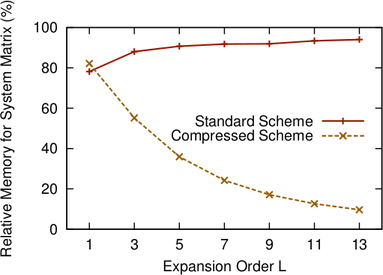
 on a three-dimensional
  -grid with
  nodes.


 for the fully set up system matrix and the proposed
compressed matrix scheme. Both the full system of linear equations and the condensed
system with odd order unknowns eliminated in a preprocessing step are compared.
for the fully set up system matrix and the proposed
compressed matrix scheme. Both the full system of linear equations and the condensed
system with odd order unknowns eliminated in a preprocessing step are compared.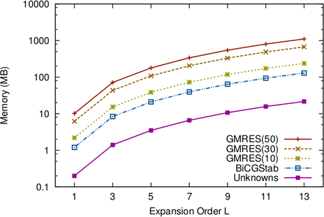
 and BiCGStab as given in Tab.