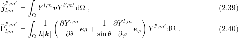
with spatial location
  , wave vector
  and time
  into
spherical harmonics
into
spherical harmonics  of the form
This chapter gives a brief introduction to the spherical harmonics expansion (SHE) method for the deterministic numerical solution of the BTE. First, the developments since the introduction of the method in the early 1990s are discussed. Connections with the new contributions presented in this work are established as much as possible. Then, the formulation of the SHE equations as proposed by Jungemann et al. [53] and later refined by Hong et al. [42] is presented, which is also the foundation for the contributions in subsequent chapters. The chapter closes with a comparison of the requirements on modern TCAD given in Sec. 1.2 and the current state-of-the-art of the SHE method.
First journal publications on the SHE method date back to Gnudi et al. [21] as well as Goldsman
et al. [25] in 1991. However, a precursor of the method has already been used in the PhD thesis
of Goldsman in 1989 [24]. Even though the method formally relies on an expansion of the
distribution function with spatial location , wave vector and time into
spherical harmonics of the form
 is written in spherical coordinates
  ,
,  and
and  on
equi-energy surfaces, the derivation of equations for the expansion coefficients was rather based on
perturbations of the ground state at
on
equi-energy surfaces, the derivation of equations for the expansion coefficients was rather based on
perturbations of the ground state at  than on a clean mathematical approach such as a
Galerkin scheme. Consequently, the derivation of the equations required a lot of bookkeeping.
Nevertheless, the first-order expansion was extended to the two- and multi-dimensional
case soon after [23, 110]. It is worthwhile to mention the
than on a clean mathematical approach such as a
Galerkin scheme. Consequently, the derivation of the equations required a lot of bookkeeping.
Nevertheless, the first-order expansion was extended to the two- and multi-dimensional
case soon after [23, 110]. It is worthwhile to mention the  -transform, which has
been proposed already at a very early stage in the development of the SHE method
[23].
-transform, which has
been proposed already at a very early stage in the development of the SHE method
[23].
In the mid-1990s a large number of publications dealt with the SHE method. Lin et
al. derived a Scharfetter-Gummel-type stabilization [65] for the first-order SHE method, and
coupled the SHE method for electrons with the Poisson equation and the hole continuity equation
[66]. Hennacy et al. [37, 38] extended the method to arbitrary order expansions. A comparison
of different boundary conditions has been carried out by Schroeder et al. [92]. Vecchi et al.
[105] proposed an efficient solution scheme based on a multigrid-like refinement of the
grid near the conduction band edge. Moreover, a decoupling of the system of linear
equations after discretization is discussed for the case that only one inelastic scattering
mechanism with constant energy transfer is considered. Even though the techniques
presented therein differ substantially from those discussed in Chap. 6 and Chap. 7,
the crucial role of inelastic scattering for the coupling structure and methods for the
resolution enhancement near the band edge have been discussed already. The same group
proposed a scheme for incorporating full-band effects for both the conduction and
the valence band [107, 106]. The publication by Rahmat et al. [78] observed that
the spatial terms of the SHE equations can be handled separately from the angular
coupling, which is the key observation used throughout Chap. 4. However, this separation
was given as an implementation hint for the assembly of the Jacobian matrix only,
while in Chap. 4 the system matrix is kept in a compressed form and is never set up
explicitly. The same publication also covers aspects of numerical stability and proposes an
upwinding scheme based on trial and error. The attractiveness of the SHE method for
the investigation of hot-carrier effects is reflected in publications on the inclusion of
electron-electron scattering for first-order SHE [108, 109], and by investigations of
impact ionization [22] as well as hot-electron injections [77]. Singh [97] discussed the
advantage of using inelastic scattering in order to avoid spurious oscillations in the
distribution function and proved that the resulting system matrix for first-order SHE is an
 -matrix, which ensures the positivity of the distribution function at the discrete
level.
-matrix, which ensures the positivity of the distribution function at the discrete
level.
The number of publications on the SHE method by the engineering community declined towards the end of the 20th century. Instead, publications from mathematicians increased. Ben Abdallah [2] put the first-order SHE method in context with established moment-based methods and derived high-field approximations [3]. Ringhofer proposed various expansion approaches for the BTE based on entropy functionals [82, 81, 83] and proposed an expansion of the energy coordinate into Hermite polynomials [80]. Hansen et al. [36] analyzed the SHE method for plasma physics.
In the early 2000s, Goldsman et al. [26, 35] applied a first-order SHE method to the modified
Boltzmann equation taking contributions from the Wigner equation into account. The publication
of Jungemann et al. [53] in 2006 applied the maximum entropy dissipation scheme
developed by Ringhofer to a discretization in  -space, where
  denotes kinetic
energy, and put arbitrary order expansions on solid grounds by using a Galerkin scheme
for the angular components. Furthermore, higher-order expansions were shown to be
required for devices in the nanometer regime, a box-integration scheme suitable also for a
certain class of unstructured grids was proposed, and the need for good preconditioners
in order to obtain convergence of iterative solvers was discussed. Hong et al. [44]
presented the first arbitrary-order implementation of the SHE method in two spatial
dimensions in 2008, refined the numerical scheme in 2009 to cover magnetic fields,
and re-introduced the
denotes kinetic
energy, and put arbitrary order expansions on solid grounds by using a Galerkin scheme
for the angular components. Furthermore, higher-order expansions were shown to be
required for devices in the nanometer regime, a box-integration scheme suitable also for a
certain class of unstructured grids was proposed, and the need for good preconditioners
in order to obtain convergence of iterative solvers was discussed. Hong et al. [44]
presented the first arbitrary-order implementation of the SHE method in two spatial
dimensions in 2008, refined the numerical scheme in 2009 to cover magnetic fields,
and re-introduced the  -transform in order to preserve numerical stability in the
deca-nanometer regime [42]. A full-band SHE of the valence band was presented by Pham
et al. [73]. Recently, Matz et al. [69, 45] presented a fitted band structure for the
conduction band for use with the SHE method, which further increases the accuracy of the
SHE method, but at the expense of considerably increased computational costs. In
2011, Jin et al. [48] proposed a simplified method for the inclusion of full-band effects,
which preserves the accuracy of the fitted band structure without notably increasing
the computational effort. Hong et al. [43] also extended the SHE method to obey
Pauli’s exclusion principle, while Pham et al. [75, 74, 76] coupled the Schrödinger
equation with a SHE method of reduced dimensionality for multi-subband solutions of
PMOSFETs.
-transform in order to preserve numerical stability in the
deca-nanometer regime [42]. A full-band SHE of the valence band was presented by Pham
et al. [73]. Recently, Matz et al. [69, 45] presented a fitted band structure for the
conduction band for use with the SHE method, which further increases the accuracy of the
SHE method, but at the expense of considerably increased computational costs. In
2011, Jin et al. [48] proposed a simplified method for the inclusion of full-band effects,
which preserves the accuracy of the fitted band structure without notably increasing
the computational effort. Hong et al. [43] also extended the SHE method to obey
Pauli’s exclusion principle, while Pham et al. [75, 74, 76] coupled the Schrödinger
equation with a SHE method of reduced dimensionality for multi-subband solutions of
PMOSFETs.
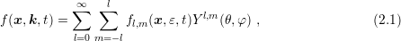
The SHE equations are derived in the following. The calculations mostly follow those given by Jungemann et al. [53]. For reasons of clarity, function arguments are omitted whenever appropriate. Furthermore, the explicit inclusion of the Herring-Vogt transform as well as the inclusion of a magnetic field, which are detailed by Hong et al. [42], are avoided. For details on spherical harmonics the reader is referred to the literature [18, 41, 20], and for the particular phase factors used within this thesis to [86].
The derivation is carried out for an expansion of the distribution function  into
spherical harmonics as in (2.1) on equi-energy surfaces, which requires that the mapping
into
spherical harmonics as in (2.1) on equi-energy surfaces, which requires that the mapping
 is a bijection. For a given distribution function
  , the expansion coefficients are
obtained from projections:
, the expansion coefficients are
obtained from projections:
 | (2.2) |
Here,  denotes the unit sphere, and the generalized density of states including spin degeneracy
in the absence of magnetic fields is given by
denotes the unit sphere, and the generalized density of states including spin degeneracy
in the absence of magnetic fields is given by

It is important to keep in mind that the spherical harmonics are not orthogonal with respect to the bilinear form

 does not depend on the angles. For this
reason, one may alternatively expand the generalized distribution function
does not depend on the angles. For this
reason, one may alternatively expand the generalized distribution function  and use the standard inner product on the unit sphere, which is the approach taken
by Jungemann et al. [53]. In the following, however, an expansion of
and use the standard inner product on the unit sphere, which is the approach taken
by Jungemann et al. [53]. In the following, however, an expansion of  is carried
out, but differences to an expansion with respect to
is carried
out, but differences to an expansion with respect to  are pointed out on a regular
basis.
are pointed out on a regular
basis.
One pitfall in the derivation of the SHE equations for an expansion of  is related to the
representation (2.2) for a given distribution function
is related to the
representation (2.2) for a given distribution function  . The BTE is to be solved for an unknown
distribution function
. The BTE is to be solved for an unknown
distribution function  , hence
  is not obtained directly from a given function. Instead, the
unknown distribution function
is not obtained directly from a given function. Instead, the
unknown distribution function  is expanded into spherical harmonics, which ultimately results
in equations for the expansion coefficients
is expanded into spherical harmonics, which ultimately results
in equations for the expansion coefficients  . Keeping in mind that the spherical
harmonics are not necessarily orthogonal with respect to the bilinear form (2.4), there
holds
. Keeping in mind that the spherical
harmonics are not necessarily orthogonal with respect to the bilinear form (2.4), there
holds

 only in the case of a generalized density of states
independent of the angles, i.e.
only in the case of a generalized density of states
independent of the angles, i.e.  , but not for the general case of an angular
dependency.
, but not for the general case of an angular
dependency.
In order to derive a set of equations for the expansion coefficients  for an unknown
function
for an unknown
function  known to fulfill the BTE (1.1), one can proceed in two ways. The first possibility is to
insert the expansion into the BTE and then project the resulting equation onto spherical
harmonics, while the second possibility is to first project the BTE and then insert the expansion
of
known to fulfill the BTE (1.1), one can proceed in two ways. The first possibility is to
insert the expansion into the BTE and then project the resulting equation onto spherical
harmonics, while the second possibility is to first project the BTE and then insert the expansion
of  . Both operations are linear and the BTE itself is linear when using linear scattering
operators only, thus both methods yield the same result provided that all required exchanges of
summation and integration are valid. Since the latter method leads to less notational
clutter, first a projection of the BTE onto each of the spherical harmonics
. Both operations are linear and the BTE itself is linear when using linear scattering
operators only, thus both methods yield the same result provided that all required exchanges of
summation and integration are valid. Since the latter method leads to less notational
clutter, first a projection of the BTE onto each of the spherical harmonics  of the
form
of the
form

 are detailed in the following term-by-term. Function
arguments are usually suppressed to increase the legibility of the expressions.
are detailed in the following term-by-term. Function
arguments are usually suppressed to increase the legibility of the expressions.
 : Since the time derivative can be pulled in front of the projection integral, one
immediately obtains
: Since the time derivative can be pulled in front of the projection integral, one
immediately obtains ![∂[f ]l,m ∕∂t](diss-et233x.png) , where
, where
![∫
[f ]l,m := Yl,mf Zd Ω (2.7)
Ω](diss-et234x.png)
 as outlined above.
 : Similar to the previous term, the gradient with respect to the spatial coordinate
 can be pulled in front of the integral, thus leading to


 : In contrast to the other terms, the derivative cannot be pulled out of the
projection integral. Since the gradient with respect to the wavevector
: In contrast to the other terms, the derivative cannot be pulled out of the
projection integral. Since the gradient with respect to the wavevector  of the distribution
function
of the distribution
function  would lead to problems for a separation of
  and
and  after inserting the
expansion (2.1), an integration by parts is carried out. To avoid formal difficulties with the delta
distribution, the projection is in addition first multiplied with a smooth test function
after inserting the
expansion (2.1), an integration by parts is carried out. To avoid formal difficulties with the delta
distribution, the projection is in addition first multiplied with a smooth test function  and
integrated over energy:
and
integrated over energy:
| ∫ 0∞ψ(ε) |  ∫
Bδ(ε − ε(k))Y l,m ∫
Bδ(ε − ε(k))Y l,m ⋅∇kfdkdε ⋅∇kfdkdε | ||
=  ⋅∫
Bψ(ε(k))Y l,m∇
kfdk ⋅∫
Bψ(ε(k))Y l,m∇
kfdk | |||
= − ⋅∫
B∇k(ψ(ε(k))Y l,m)fdk ⋅∫
B∇k(ψ(ε(k))Y l,m)fdk | |||
= − ⋅∫
B ⋅∫
B![[ ]
∂ψ-∇ ε(k )Y l,m + ψ (ε(k))∇ Y l,m
∂ε k k](diss-et251x.png) fdk fdk |
 in
in  -space is given by

 ,
,  and
and  denote the unit vectors in
  ,
,  and
and  -direction, respectively. The
invariance of spherical harmonics with respect to the radial direction and the relation
-direction, respectively. The
invariance of spherical harmonics with respect to the radial direction and the relation
 leads to
| ∫ 0∞ψ(ε) |  ∫
Bδ(ε − ε(k))Y l,m ∫
Bδ(ε − ε(k))Y l,m ⋅∇xfdkdε ⋅∇xfdkdε | ||
= −F ⋅∫
0∞ ∫
ΩY l,mvfZdΩdε ∫
ΩY l,mvfZdΩdε | |||
−F ⋅∫
0∞ψ(ε)∫
Ω  fZdΩdε fZdΩdε | |||
= −F ⋅∫
0∞ jl,m + ψΓl,mdε jl,m + ψΓl,mdε | |||
= F ⋅∫
0∞ψ dε , dε , |

 can be taken ‘arbitrarily’, one obtains

 : The scattering operator in the low-density approximation is considered, which
neglects the nonlinearity introduced by Pauli’s exclusion principle:
: The scattering operator in the low-density approximation is considered, which
neglects the nonlinearity introduced by Pauli’s exclusion principle:

 in front, which is then
included in the denominator of the scattering rates. In this work, the sample volume
in front, which is then
included in the denominator of the scattering rates. In this work, the sample volume  is not
written explicitly. To allow for several different scattering processes like acoustical
and optical phonon scattering, the index
is not
written explicitly. To allow for several different scattering processes like acoustical
and optical phonon scattering, the index  is used for writing the scattering rate
as
is used for writing the scattering rate
as

 denote the initial and the final state respectively.
The minus sign stands for emission of energy and the plus sign for absorption. In the case of
multiple energy bands, summation over all energy bands has to be added to (2.14), cf. [53]. In
the following only a single band is considered, a generalization to multiple bands mainly consists
of a summation over all energy bands involved.
denote the initial and the final state respectively.
The minus sign stands for emission of energy and the plus sign for absorption. In the case of
multiple energy bands, summation over all energy bands has to be added to (2.14), cf. [53]. In
the following only a single band is considered, a generalization to multiple bands mainly consists
of a summation over all energy bands involved.
The scattering integral is split into an in-scattering term


 | (2.17) |
where
 | (2.18) |
Similarly, the out-scattering term is evaluated as

 | (2.20) |
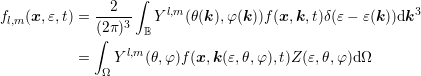
A considerable simplification can be achieved if the transition rate is assumed to be velocity
randomizing, i.e. the coefficient  in (2.14) depends only on the initial and final energy, but
not on the angles. This allows for rewriting (2.18) as
in (2.14) depends only on the initial and final energy, but
not on the angles. This allows for rewriting (2.18) as
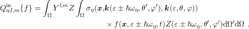
![∫ ∫
in,VR l,m ′ ′ ′
Q η,l,m {f} = ση(x,ε ± ℏωη,ε) Y Zd Ω f(x,ε± ℏωη,t)Z (ε± ℏω η,θ,φ )dΩ
Ω Ω
= ση(x,ε ± ℏωη,ε)Zl,m (ε)[f-(x,-ε±-ℏω-η)]0,0-,
Y0,0](diss-et286x.png) | (2.21) |
where (2.7) was used and  denotes the orthonormal projection of the generalized density
of states onto the spherical harmonic
denotes the orthonormal projection of the generalized density
of states onto the spherical harmonic  using the standard inner product on the sphere. In
the case of spherical bands,
using the standard inner product on the sphere. In
the case of spherical bands, ![[f] = f Z
0,0 0,0](diss-et289x.png) and thus only
and thus only  is coupled into the balance
equation for
is coupled into the balance
equation for  .
.
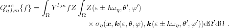
With the assumption of velocity-randomization, the out-scattering term can be simplified to
![∫ ∫
out,VR l,m ′
Q η,l,m {f} = ση(x,ε,ε ± ℏωη) × Y fZd Ω × Z (ε± ℏω η,θ,φ)dΩ
∑ Ω Ω
= ση(x,ε,ε± ℏω η)[f]l,m Z0,0(ε±-ℏ-ωη)-.
η Y0,0](diss-et292x.png) | (2.22) |
Thus, the out-scattering term is proportional to  in the case of a spherically symmetric
density of states
in the case of a spherically symmetric
density of states  . If an expansion of the generalized distribution function
  is carried
out instead of an expansion of
is carried
out instead of an expansion of  , then the out-scattering term is proportional to
  irrespective of any spherical symmetry of
  .
.
Summing up, the full projected scattering operator using velocity randomization (VR) is thus given by
![[
QVR {f} = --1- ∑ Z (ε)σ (x, ε± ℏω ,ε)[f(x,ε ± ℏω ,t)]
l,m Y 0,0 η l,m η η η 0,0
]
− [f]l,m(x,ε,t)ση(x,ε,ε∓ ℏωη)Z0,0(ε ∓ ℏωη) .](diss-et299x.png) | (2.23) |
Even though the scattering operator after projection is not an integral operator any longer,
shifted arguments on the right hand side show up whenever inelastic collisions characterized by
 are considered.
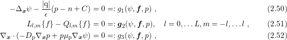
Collecting all individual terms, we obtain the system of equations for the BTE upon projection onto spherical harmonics on equi-energy surfaces under the assumption of velocity randomization:
![∂[f] (∂j )
---l,m--+ ∇x ⋅jl,m (x, ε,t) + F ⋅ ---l,m − Γ l,m =
∂t ∑ [ ∂ε
= -1-- Zl,m(ε)ση(x,ε ± ℏωη,ε)[f ]0,0(x, ε± ℏωη,t)
Y 0,0 η
]
− [f]l,m (x,ε,t)ση(x,ε,ε∓ ℏω η)Z0,0(ε∓ ℏ ωη)](diss-et301x.png) | (2.24) |
It is worthwhile to note that an expansion of  instead of
  leads to the same system of
equations when replacing
leads to the same system of
equations when replacing ![[f]](diss-et304x.png) with
with  .
.
 -Transform and MEDS
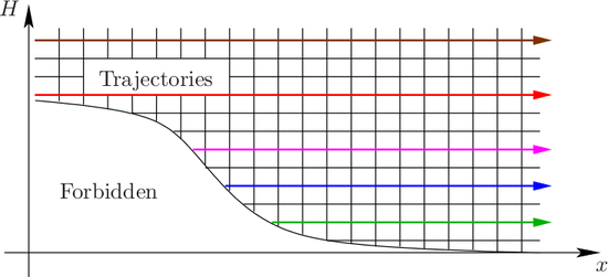
A discretization of the system (2.24) in  -space leads to spurious oscillations for very small
devices, because the grid is not aligned with the trajectories of carriers in free flight. The
numerical stability can be improved substantially by a transformation from kinetic energy
-space leads to spurious oscillations for very small
devices, because the grid is not aligned with the trajectories of carriers in free flight. The
numerical stability can be improved substantially by a transformation from kinetic energy  to
total energy
to
total energy  , because trajectories are then given by
  . The price to pay for the
increased numerical stability is the additional effort for handling the band-edge given by
. The price to pay for the
increased numerical stability is the additional effort for handling the band-edge given by  ,
because the simulation domain needs to be adjusted with every update of the electrostatic
potential.
,
because the simulation domain needs to be adjusted with every update of the electrostatic
potential.
 .
.
The  -transform was suggested already soon after the SHE method had been
introduced [23]. In the following, the application of the
-transform was suggested already soon after the SHE method had been
introduced [23]. In the following, the application of the  -transform to (2.24) in the way
proposed by [42] is shown. Consider a variable transformation from
-transform to (2.24) in the way
proposed by [42] is shown. Consider a variable transformation from  to
to  by
by

 can be an arbitrary function of
  and
and  is the signed charge of the carrier. The
system (2.24) is then transformed to
is the signed charge of the carrier. The
system (2.24) is then transformed to
![∂[f]l,m-+ ∇ ˜x ⋅jl,m + [F + ∇xH ]⋅ ∂jl,m − F ⋅Γ l,m
∂t [ ∂H
= --1-∑ Z σ (˜x, H ± ℏω ,H )[f] (x˜, H ± ℏω ,t)
Y0,0 η l,m η η 0,0 η
]
− [f]l,mσ η(˜x, H,H ∓ ℏωη)Z0,0(H ∓ ℏωη) .](diss-et322x.png) | (2.26) |
Since the force term is given by
![F = − ∇x [Ec (x )+ qψ (x )] , (2.27)](diss-et323x.png)
 is the position-dependent valley minimum and
  the electrostatic potential, the
derivative of
the electrostatic potential, the
derivative of  with respect to
  is eliminated by the choice

 implies that
  refers to the total energy. The
  -transformed system is
thus given by
-transformed system is
thus given by
![[
∂[f]l,m-+ ∇ ⋅j − F ⋅Γ = -1--∑ Z σ (x, H ± ℏω ,H )[f] (x,H ± ℏω ,t)
∂t x l,m l,m Y0,0 l,m η η 0,0 η
η ]
− [f]l,mσ η(x, H,H ∓ ℏωη)Z0,0(H ∓ ℏωη) ,](diss-et332x.png) | (2.29) |
where  is written instead of
  .
.
Inserting the expansion (2.1) into (2.29) yields
![l′,m ′ ∂fl′,m ′ l′,m′ l′,m ′
[Y ]l,m--∂t-- + ∇x ⋅jl,m fl′,m ′ − F ⋅Γ l,m fl′,m′
1 ∑ [ ′ ′
= ---- Zl,mση(x, H ± ℏωη,H )[Yl,m ]0,0fl′,m′(x,H ± ℏωη,t)
Y0,0 η
l′,m ′ ]
− [Y ]l,mfl′,m′ση(x,H, H ∓ ℏω η)Z0,0(H ∓ ℏω η) ,](diss-et335x.png) | (2.30) |
where Einstein’s summation convention over pairs of upper and lower indices is employed. The coefficients
![∫
l′,m ′ l,m l′,m′
[Y ]l,m := Y Y ZdΩ , (2.31)
′ ′ ∫Ω ′ ′
jll,,mm := Y l,mvY l,m Zd Ω , (2.32)
∫Ω ( )
l′,m ′ -1-- ∂Yl,m-- -1--∂Y-l,m- l′,m ′
Γ l,m := Ω ℏ|k | ∂θ eθ + sin θ ∂φ eφ Y Zd Ω (2.33)](diss-et336x.png)
The even part of the carrier distribution function can be associated with densities like the
carrier density or the energy density, while the odd part of the carrier distribution function is
viewed as fluxes. To improve numerical stability, these fluxes need to be stabilized [82]. Based on
entropy dissipation principles, Ringhofer proposed to multiply the projected SHE equations with
the entropy function 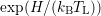 , where
  is the Boltzmann constant and
  denotes
lattice temperature, and to take the negative adjoint form of the projected equations for odd
denotes
lattice temperature, and to take the negative adjoint form of the projected equations for odd  [82]. While the multiplication with the entropy function is crucial for a formulation based on
kinetic energy as in (2.24) and [53], it is just a constant factor in a formulation based on total
energy such as (2.30). Therefore, it is sufficient to simply take the negative adjoint operator
[42]:
[82]. While the multiplication with the entropy function is crucial for a formulation based on
kinetic energy as in (2.24) and [53], it is just a constant factor in a formulation based on total
energy such as (2.30). Therefore, it is sufficient to simply take the negative adjoint operator
[42]:
![′ ′ ∂fl′,m′ ( ′ ′ ) ′ ′
l even : [Yl,m ]l,m----- + ∇x ⋅ jll,,mm fl′,m′ − F ⋅Γ ll,,mm fl′,m ′
∂t ∑ [
= -1-- Zl,m ση(x,H ± ℏωη,H )[Y l′,m ′]0,0fl′,m′(x,H ± ℏω η,t)
Y0,0 η
l′,m′ ]
− [Y ]l,mfl′,m ′σ η(x, H,H ∓ ℏωη)Z0,0(H ∓ ℏωη) ,](diss-et341x.png) | (2.34) |
![l odd : [Y l′,m ′]l,m ∂fl′,m-′+ jl′,m′⋅∇xfl ′,m′ + F ⋅ ˆΓ l′,m′fl′,m ′
∂t l,m [ l,m
-1--∑ l′,m′ ′ ′
= Y0,0 Zl,m ση(x,H ± ℏω η,H )[Y ]0,0fl,m (x,H ± ℏωη,t)
η ]
− [Y l′,m ′]l,mfl′,m′ση(x,H, H ∓ ℏ ωη)Z0,0(H ∓ ℏωη) ,](diss-et342x.png) | (2.35) |
where Einstein’s summation convention over pairs of upper and lower indices is employed. The
coupling coefficients ![[Yl′,m′]l,m](diss-et343x.png) and
and  are self-adjoint and thus unchanged, while
  is
given by
is
given by

It is worthwhile to compare (2.34) and (2.35) with the system obtained from an expansion of

 after repeating the previous steps as
![∂gl,m- ˜ l′,m′ ˜l′,m ′
∂t + ∇x ⋅j l,m gl′,m′ − F ⋅Γ l,m gl′,m′
-1-∑ [
= Y0,0 Zl,mσ η(x, H ± ℏω η,H )g0,0(x,H ± ℏωη,t)
η ]
− g σ (x,H, H ∓ ℏ ω )Z (H ∓ ℏ ω )
l,m η η 0,0 η](diss-et349x.png) | (2.38) |
with coupling coefficients
 are obtained in the same way by taking the negative adjoint form. If the
density of states
are obtained in the same way by taking the negative adjoint form. If the
density of states  does not show an angular dependence, the two approaches are equivalent,
otherwise the truncated expansions will yield different results in general. To the knowledge of the
author, a systematic comparison of the formulations (2.34) and (2.35) with (2.38) for nonspherical
energy bands has not been carried out yet.
does not show an angular dependence, the two approaches are equivalent,
otherwise the truncated expansions will yield different results in general. To the knowledge of the
author, a systematic comparison of the formulations (2.34) and (2.35) with (2.38) for nonspherical
energy bands has not been carried out yet.
The system (2.34) and (2.35) consists of an infinite number of equations due to an expansion
of  of the form (2.1). The conforming Galerkin procedure for obtaining a finite set of equations
is to consider a truncated expansion
of the form (2.1). The conforming Galerkin procedure for obtaining a finite set of equations
is to consider a truncated expansion
 , and to consider only a finite subset of
the projected equations. The typical choice
, and to consider only a finite subset of
the projected equations. The typical choice  and
and  for the
projected equations is used in the remainder of this thesis, hence the number of unknown
expansion coefficients and the number of equations agree. Otherwise, approximations in the
least-squares sense for the over- or under-determined system would have to be considered.
However, least-squares problems lead to additional computational effort compared to the
solution of a linear system, thus no investigations have been carried out in that direction
yet.
for the
projected equations is used in the remainder of this thesis, hence the number of unknown
expansion coefficients and the number of equations agree. Otherwise, approximations in the
least-squares sense for the over- or under-determined system would have to be considered.
However, least-squares problems lead to additional computational effort compared to the
solution of a linear system, thus no investigations have been carried out in that direction
yet.
So far, the force term  has been considered to be a given quantity. In a homogeneous material
it is linked to the electrostatic potential
has been considered to be a given quantity. In a homogeneous material
it is linked to the electrostatic potential  by
by 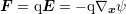 , where
  denotes the signed
charge of the particle and
denotes the signed
charge of the particle and  the electric field. With Gauss’ Law, a scalar permittivity
  and
the charge density
and
the charge density  , where
  and
and  denote the density of holes and electrons
respectively, and
denote the density of holes and electrons
respectively, and  refers to the density of fixed charges in the material, the Poisson
equation
refers to the density of fixed charges in the material, the Poisson
equation

Since the carrier density depends on the solution of the BTE, which in turn depends on the
solution of the Poisson equation, a self-consistent solution of both equations has to be found.
Even though both equations are linear in their unknowns, the coupling is nonlinear due to the
inner product of the force  with the gradient
  of the distribution function with respect to
the wave vector
of the distribution function with respect to
the wave vector  . Consequently, a nonlinear iteration scheme has to be employed for the
solution of the coupled system
. Consequently, a nonlinear iteration scheme has to be employed for the
solution of the coupled system
Given the iterates  ,
,  and
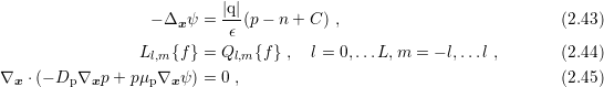
and  for the potential, electron and hole density respectively,
updates can be obtained by solving the equations (2.43), (2.44), and (2.45) sequentially in a
Gauss-Seidel-type manner [32]:
for the potential, electron and hole density respectively,
updates can be obtained by solving the equations (2.43), (2.44), and (2.45) sequentially in a
Gauss-Seidel-type manner [32]:
In its simplest form, the Gummel iteration diverges in most cases due to the exponential dependence of the carrier concentrations on the potential.
The convergence behavior can be improved substantially by considering the dependencies
 and
and  , where
  and
and  denote the quasi-Fermi potentials of electrons and holes respectively and
 is the thermal voltage. A linearization leads to the damped Poisson equation for
 :
:

The damping parameter  allows for additional control of the damping. Typical values are
about
allows for additional control of the damping. Typical values are
about  and may be chosen differently for each iteration. In order to ensure a reduction of the
residual, an additional control of
and may be chosen differently for each iteration. In order to ensure a reduction of the
residual, an additional control of  can be employed, where e.g. subsequent trials
 for
for  are chosen until the residual in the current step is reduced
[16].
are chosen until the residual in the current step is reduced
[16].
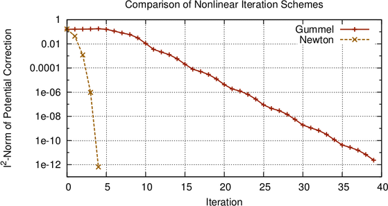
A typical convergence plot for an undamped modified Gummel iteration ( ) is depicted
in Fig. 2.2. Typical features are the almost constant potential update during the first
iterations, and the nonuniform reduction of the potential correction in later iteration steps.
These features are more pronounced for more complicated devices under higher bias.
) is depicted
in Fig. 2.2. Typical features are the almost constant potential update during the first
iterations, and the nonuniform reduction of the potential correction in later iteration steps.
These features are more pronounced for more complicated devices under higher bias.
 -diode.
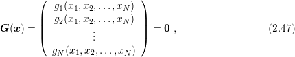
The standard method for the solution of nonlinear systems of equation is Newton’s method. The big advantage over many other methods is the quadratic convergence sufficiently close to the true solution. For a system of equations of the form
 to the true solution is determined by

 of
of  is given by
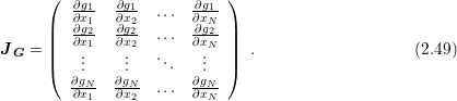
 . The method fails if the Jacobian matrix does not have full
rank, which is, however, unlikely in practice due to the regularizing effect of round-off
errors.
. The method fails if the Jacobian matrix does not have full
rank, which is, however, unlikely in practice due to the regularizing effect of round-off
errors.
A Newton method for the system (2.43)-(2.45) can be derived by writing the system in the form
 for some maximum expansion order
  . The Jacobian matrix is
then obtained as
. The Jacobian matrix is
then obtained as

 : The electron density is obtained from the distribution function as


 does not show an angular dependence, a nonzero derivative is obtained for
  only.
only.
 : Here, the derivative of the SHE equations (2.34) and (2.35) with respect to
the potential
: Here, the derivative of the SHE equations (2.34) and (2.35) with respect to
the potential  need to be taken. Since most terms depend on the kinetic energy
  , which for a
fixed total energy
, which for a
fixed total energy  depends on the potential
  , the derivative is very elaborate. For the sake
of brevity, only the derivative of the generalized current density term
, the derivative is very elaborate. For the sake
of brevity, only the derivative of the generalized current density term  is outlined
explicitly:
is outlined
explicitly:

 refers to the signed charge of the carrier. In the same
way derivatives of the terms
refers to the signed charge of the carrier. In the same
way derivatives of the terms  ,
,  and
and  are computed. The force term is
handled in the same way as for the hole continuity equation. For the case that no
analytical expression for
are computed. The force term is
handled in the same way as for the hole continuity equation. For the case that no
analytical expression for  ,
,  or
or  is available, a discrete differential quotient is
taken.
is available, a discrete differential quotient is
taken.
In practice, the Newton scheme will be used together with a damping scheme similar to the one
discussed for the Gummel iteration. The existence of a damping parameter  leading to a
reduction of the overall residual norm is ensured under reasonable assumptions about the system
of equations.
leading to a
reduction of the overall residual norm is ensured under reasonable assumptions about the system
of equations.
An examplary convergence plot for the Newton method is given in Fig. 2.2. The quadratic convergence is readily visible and leads to a much smaller number of iterations compared to the modified Gummel method.
Now as the SHE equations are derived, the state-of-the-art for the SHE method – excluding the author’s own contributions presented in the remainder of this thesis – is compared to the requirements for modern TCAD established in Sec. 1.2.
The issues raised in terms of the resolution of complicated domains as well as in
the use of computational resources will be addressed in the remainder of this thesis.
Chap. 5 discusses the use of unstructured triangular and tetrahedral meshes for the SHE
method. Chap. 6 addresses the quadratically increasing computational costs of the
SHE method with the expansion order  . In Chap. 7 a parallel preconditioner is
developed, which enables the efficient use of modern many- and multi-core computing
architectures.
. In Chap. 7 a parallel preconditioner is
developed, which enables the efficient use of modern many- and multi-core computing
architectures.