 and
and  denote
the position vector of all nuclei and all electrons, respectively. For a system containing
denote
the position vector of all nuclei and all electrons, respectively. For a system containing  will be 3
 will have 3

The degradation mechanisms discussed in this text proceed via chemical or electrochemical reactions at defects in the oxide or at the semiconductor-oxide interface. This chapter reviews the theories of theoretical and physical chemistry that are relevant for the applications presented in the later chapters, starting from the highest level of detail and moving to the less detailed but computationally more efficient macroscopic descriptions. Most of the concepts presented in this chapter are much more generally applicable than just to describe the dynamics of oxide defects. Examples are given to link those concepts to the context of the present application.
The theory employed in the present work rests upon the fundament of physical chemistry,
sometimes also referred to as “low energy physics”, which is applicable to the processes
dominating our everyday experience like the dynamics of fluids and gases, electrical and
thermal conduction, and chemical reactions. In contrast to high energy physics, where
subatomic particles and at least three of the four fundamental interactions have to be
considered, the central actors in physical chemistry are electrons and nuclei which only interact
through electrostatic forces. The theoretical foundation of quantum chemistry thus lies in the
Schrödinger equation of the system of electrons and nuclei. In the following, and denote
the position vector of all nuclei and all electrons, respectively. For a system containing will be 3 will have 3
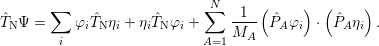
The Schrödinger equation for the system of electrons and nuclei is [88, 90, 91]
 | (2.1) |
where Ψ(
 ) is called the
 | (2.2) |
is the Hamiltonian of the system, which is sometimes also termed the
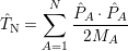
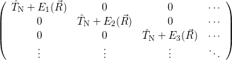
The Born-Oppenheimer approximation relies on the fact that the mass of even the lightest nuclei exceeds the electron mass by orders of magnitude. In order to make use of this property, Born and Oppenheimer rewrote the molecular Hamiltonian as
 | (2.8) |
with
=  | (2.9) | |
=     | (2.10) | |
=  
| (2.11) |
 | (2.12) |
Although this is an eigenproblem in the electronic degrees of freedom, the results depend
parametrically on the position of the nuclei. The higher order elements of the series expansion show
that the expectation value of the energy  ) associated with the electronic state
  ;
; ) will
act as a potential energy on the nuclei. Thus, the molecular wave function is obtained
as
) will
act as a potential energy on the nuclei. Thus, the molecular wave function is obtained
as
 | (2.13) |
where  ;
; ) is one of the solutions of (2.12) and
  ) is determined from
 | (2.14) |
This approximation implicitly assumes that the electronic quantum number is not affected by the
momentum of the nuclei, which means that the nuclei are assumed to move slowly enough that the
electrons can adjust  ) is the
  ) of the lowest electronic state
  ;
; ), which is the dominant state in thermal
equilibrium.
), which is the dominant state in thermal
equilibrium.
The original derivation of Born and Oppenheimer [88, 90] was restricted to molecules in which the potential energy surface was essentially a quadratic function with the nuclei moving around the minimum. Interestingly, it also gives very accurate results for situations where these conditions are not even approximately fulfilled [92, 90]. This behavior and also the breakdown of the approximation can be understood using an improved approach that is discussed later in Sec. 2.9.1.
| Figure 2.1: | Illustration of the dependence
of different electronic states on the nuclear
configuration. The adiabatically adjusting
energies of the electronic states act as potential
for the nuclei. Different electronic states may
give rise to drastically different potentials. For
example, while the potentials |
In summary, the essence of the Born-Oppenheimer approximation is that due to the large difference in masses, the heavy nuclei are standing still from the perspective of the electrons. The electrons will thus adjust their orbit instantaneously to the motion of the nuclei and the energy of this orbit acts back as a potential on the nuclei. The resulting separation of the electronic and the nuclear degrees of freedom is, however, only a slight improvement from the perspective of solubility, as a typical solid or molecule still contains too many electrons and ions for an exact solution of (2.12) and (2.14). However, both the electronic as well as the nuclear problem can be greatly simplified by the exploitation of inherent symmetries and some well-defined approximations.
The solution of the electronic many-particle problem arising from the Born-Oppenheimer
approximation is a classic topic of quantum chemistry, and a multitude of approaches exist using
different approximations. Depending on the size of the system and the available computational
resources, different levels of sophistication can be employed to calculate the potential energy surface of
a molecule or a solid. While the simplest approaches employ analytic potentials which try to mimic
the shape of the electronic energy, the more sophisticated approaches actually attempt to solve the
electronic Schrödinger equation (2.12) for its ground (and sometimes also for an excited) state. The
latter methods are referred to as
| Figure 2.2: | An intuitive picture of the self-consistent field approach. Instead of considering all the interactions between all particles (left), the problem is reformulated as a system of isolated particles moving in a mean field (right). |
For all but the smallest systems, an exact solution of the electronic Schrödinger equation is
computationally unfeasible, as the dimensionality of the problem increases linearly with the number of
particles, leading to an exponential increase in computational complexity. The first approach to
the solution of the many-electron problem for isolated atoms was reported by Hartree
in three papers in 1928 [93, 94, 95]. His approach, described in the second part of the
series, was termed ‘self-consistent field method’ as it approximates the electron-electron
interaction through an effective potential
 | (2.15) |
The formulation of Hartree’s method initially followed physical intuition rather than a mathematical derivation. Its connection to the many-body Schrödinger equation was clarified later as a variational determination of the ground state using a product-wave function ansatz.
 | (2.16) |
A central problem of this ansatz is that it does not have the required fermionic symmetries upon particle exchange [96, 97, 98]. An improved description was found by Fock using a properly symmetrized ansatz, which can be written in a compact form as determinant in which the single-particle wave function is the same along a column and the particle coordinate is the same along a row.
 | (2.17) |
Following the same basic steps as in the Hartree-method again leads to an effective single-particle
problem, with an additional self-consistent non-local potential 
 | (2.18) |
The resulting method was named Hartree-Fock self-consistent field method, the new term in the equation is usually called exchange- or Fock-operator1 . The Hartree-Fock self-consistent field method gives good results in many situations and is a standard method of quantum chemistry. The wave function resulting from the method as well as the total (ground state) energy are physically relevant within the bounds of the approximation, in contrary to the density functional approach which is discussed below. Although it is considered a reasonable starting point, the accuracy of the theory is limited due to the neglect of electronic correlation [96, 97]. A popular method that improves on this situation is the Møller-Plesset perturbation series, which brings correlation into the Hartree-Fock-Hamiltonian using a perturbation approach that dramatically improves the accuracy for some systems [99, 97].
Despite their sound theoretical foundation and the good accuracy of the perturbation
approach, Hartree-Fock based methods are rarely used for large molecules or solid-state
problems due to the large computational effort arising from the non-local exchange operator
(
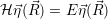
Density functional theory is a more mathematical approach to the many-body problem. It is based on the findings by Hohenberg and Kohn, which state that
From these two findings it follows that the exact ground state energy of the (3
 | (2.19) |
that has the same ground state density and energy as the interacting system. All exchange and
correlation effects of the interacting system are represented in the auxiliary system through the
effective local potential 
The most accurate methods available today are the diffusion and variational quantum Monte Carlo methods, and the configuration-interaction (CI) or coupled-cluster (CC) methods [96, 97]. These methods are able to appropriately handle correlation effects and are often used as a high-accuracy reference to benchmark self-consistent field methods. However, due to their vast computational demand those methods are usually limited to very small molecules or require massively parallel computers with thousands of CPUs. For the present work, these methods are way too expensive and also more accurate than necessary, considering the various approximations that have to be made.
The broad class of empirical electronic structure methods offers inexpensive, yet accurate solutions to various problems, especially in the field of microelectronics research. The level of physical accuracy here ranges from the classic semi-empirical quantum chemistry methods (CNDO, MNDO, PM3, …) [97] over tight-binding methods, which use a Hamiltonian that is built from analytic expressions [96], to the simplest empirical molecular dynamics potentials, which are based on analytical functions of the positions of the nuclei.
Semi-empirical quantum chemistry methods use a Hartree-Fock-based Hamiltonian, which replaces
some of the more expensive integrals with parametrizable expressions. These methods have been under
active development for decades, and are especially popular in the field of organic chemistry. The
parameters for these methods are usually calibrated to small molecules, and the standard
parametrizations have been shown to fail in the solid-state context [103, 104]. A comparison of
semi-empirical methods for the calculation of the oxygen vacancy defect in
Empirical tight-binding methods are often used for the study of the electronic structure of ideal
bulk or surface structures [96]. They have also been employed in defect studies, primarily for defects
in crystalline and amorphous silicon [106, 107, 108], but also for defects in SiO
A review of different empirical molecular dynamics potentials applied to silicon or SiO
The advantage of semiempirical methods is the inclusion of experimental input, to account
efficiently for the physics neglected in the approximations. For the study of defects in SiO
For electronic structure problems it is reasonable to treat the correlated motion of the electrons as a
second-order effect, which does not influence the basic behavior for most practical cases. For the
motion of the nuclei, an approximation like this is not possible. Vibrational states are usually heavily
correlated motions of nuclei like stretching or bending modes in molecules or phonons in a solid. A
fully quantum-mechanical treatment is again impossible due to the large number of degrees of freedom
and even a quantum Monte-Carlo-like treatment is unfeasible due to the computational effort required
to calculate the potential energy surface. It is thus necessary to either approximate the quantum
mechanical nuclear problem as a classical one or to approximate the potential energy surface as an
essentially quadratic function of the position of the nuclei so that the atomic motion can be
separated into uncoupled harmonic oscillations. The former method is broadly applied
throughout theoretical chemistry for molecules and solids and is well suited for situations where
temperatures are high enough so that quantization effects may be neglected and where
the adiabatic Born-Oppenheimer approximation holds. With respect to the BTI model
introduced in Sec. 1.5, this concerns the structural transitions 1
Once the potential energy surface for a given atomic system is known and a sufficiently accurate
description of the nuclear dynamics has been found, it is possible to calculate observable
quantities and predict the evolution of that system over time. The state of the atomic
system under consideration is fully described by the state of the electronic system, which is
usually identified by its potential energy surface, and the nuclear state, which is  ) in a
quantum-mechanical description and the instantaneous position in phase-space (
) in a
quantum-mechanical description and the instantaneous position in phase-space (
 ) —
) —  denoting
the momenta of all particles — in a classical description. In the following, these combinations of
electronic and nuclear states will be called
denoting
the momenta of all particles — in a classical description. In the following, these combinations of
electronic and nuclear states will be called
| Figure 2.3: | The potential energy surface of an atomic system typically has several minima which are separated by energetic barriers. The nuclei will spend a significant amount of time oscillating randomly around those minima and will eventually pass the barriers at time scales that are too short to be observable. Along the barriers, the configuration space can be separated into chemical states, illustrated as grey/white region. The potential energy surface could for example arise from two different bonding states of a defect, as schematically shown in the boxes. |
In order to understand chemical kinetics, it is first necessary to define in a physically
meaningful way the
Once a chemical state is defined in terms of microstates, the measurable observables are obtained from thermal averages over those microstates belonging to this chemical state. If the nuclei are treated as classical particles, those thermal averages consist of integrals over a certain potential energy surface and over the momentum-space of the nuclei, which is commonly assumed to follow the behavior of the ideal gas [112].
As mentioned above, in practical calculations it is assumed that transitions between chemical states occur instantaneously and the thermal equilibrium of the microstates in the new chemical state is established immediately. This assumption is obviously justified for transitions of the electronic subsystem, as mentioned above. Transitions between the minima of a potential energy surface or between two different electronic states are usually followed by an equilibration phase where the momentum distribution of the nuclei returns to the ideal gas distribution. This equilibration usually proceeds at time-scales of picoseconds, which is also reasonably instantaneous for most observables. However, especially for the case of hydrogen-passivated dangling bonds at the silicon surface, long-term stable vibrational modes have been reported which lead to a considerably prolonged equilibration [113]. Thus, regarding the nuclear subsystem the assumption of instantaneous transitions needs to be applied cautiously.
For the sake of completeness it is mentioned here that, as chemical states may be arbitrarily defined,
it is possible that certain microstates are part of more than one chemical state. Additionally, a
chemical state may consist of an arbitrary number of lower-level chemical states. To avoid confusion,
in the following all chemical states and reactions are
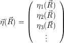
Once the chemical states and reactions that comprise the chemical system under consideration are
defined, their dynamics can be described as a random process that switches between states [114, 115].
For this purpose, the state of the chemical system is described as a vector  . Additionally, a set of
reaction channels is established, which cause the transitions between the discrete states of this vector.
Due to the unpredictable nature of the dynamics of the microstates, the time at which a reaction takes
place is not a deterministic quantity. Instead, if the chemical system is in a given state
. Additionally, a set of
reaction channels is established, which cause the transitions between the discrete states of this vector.
Due to the unpredictable nature of the dynamics of the microstates, the time at which a reaction takes
place is not a deterministic quantity. Instead, if the chemical system is in a given state 


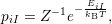
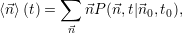
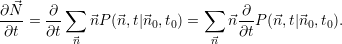
According to the theory of stochastic chemical kinetics [114, 115], the evolution of this system over time can then be described by a chemical master equation
![∂P(⃗x,t)- ∑Γ
∂t = [aγ(⃗x - ⃗νγ)P (⃗x- ⃗νγ,t)- aγ(⃗x)P (⃗x,t)],
γ=1](thesis84x.png) | (2.20) |
where 
 =
= 

 (
( at time
 (
(
| Figure 2.4: | Illustration of the example system discussed in the text.
The system exists in one of the two states     |
The master equation approach can be illustrated using the simple example of a system with two
states 


 | (2.21) |
The propensity functions
 | = |  | = 0 | (2.22) |
 | = 0 |  | = | (2.23) |
 | =   | (2.24) |
 | =   | (2.25) |
 | (2.26) |
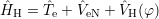
which reduces the master equation of the two-state system to
 | (2.27) |
This is the rate-equation of the two-state system, which is equivalent to the master equation for this simple example.
Within the theoretical frame work of the chemical master equation, all the microphysical details
elaborated in the previous section are now contained in the propensity functions 
The assumptions introduced above lay the foundation for the development of theoretical methods to calculate rates between chemical states. As mentioned in Sec. 2.4, the description of the nuclear state can either be classical with the full potential energy surface or quantum-mechanical with a highly idealized potential. Both approaches contain specific approximations and thus need to be cautiously applied to real-world situations. Quite generally, for reactions occurring at low temperatures the quantum-mechanical approach will be the most suitable as the effects of quantization and tunnelling may be pronounced, yet the nuclear system will be close to a minimum of the potential energy surface where idealizations are quite accurate. For reactions at higher temperatures, quantum mechanical effects will be less pronounced but the system will occupy states that are further away from the potential minima which are poorly described by the usually harmonic model Hamiltonians.
| Figure 2.5: | Illustrative example of a
potential energy surface along a reaction
path. The reaction path itself is the
optimal path on the 3 |
Barrier hopping transitions such as the structural transitions in the BTI model are reactions which the electronic system follows adiabatically and thus only change the state of the nuclear system. For the temperature ranges relevant to this document these transitions are sufficiently described using classical nuclei. This is a common working-hypothesis in practical calculations [119, 120, 112] and is sometimes supplemented with quantum mechanical corrections [112] where necessary. The microstates consist of the electronic state, which is unchanged except for the adiabatic adjustment of the electronic wave functions, and the position of the nuclear system in phase-space [119], which follows classical mechanics.
As mentioned above, for a given defect model the barrier hopping processes can in principle be described by a propagation of the microstates, i.e. the phase-space position of the nuclei. Calculations of this type are called molecular dynamics simulations [119]. However, the time range that can be treated with molecular dynamics is in the picosecond regime and can only be extended to nanoseconds for classical molecular dynamics potentials, which are not usable in defect calculations. Usual defect reactions in BTI occur in and above the microsecond regime [26, 37], which makes them rare events from a microstate perspective.
The theory employed for the calculation of rates in this picture is the 

In practice, one is usually only interested in the temperature activation for a certain transition.
Also, the thermal integrals necessary to calculate the flux through the transition state, are quite
tedious to calculate. Due to the assumption of thermal equilibrium, in which the system preferably
occupies states of lower energy, the transition will be dominated by the point of lowest
energy of the transition state. In practical calculations it is thus usually sufficient to find the
energetically optimal path between the energetic minimum point of
The charge-state transitions in the multi-state multi-phonon transition model for BTI involve the trapping of holes from the silicon valence band. These trapping events are understood as non-radiative multi-phonon (NMP) transitions. Multi-phonon, or vibronic, transitions are transitions involving a change of the electronic and the vibrational state. They play significant roles in many domains of molecular and solid state physics and have been studied extensively from both the experimental and theoretical side [91, 122, 123, 124, 125] especially for transitions at point-defects. The development of the theory of vibronic transitions is tightly linked to the development of the quantum mechanical theory of solids and molecules. As multi-phonon transitions at defects are inherently quantum-mechanical processes that are significantly influenced by a chaotic perturbation (i.e. the heat-bath), their theoretical description is a quite demanding task and usually involves strong idealizations.
The first theory capable of explaining the behavior of molecules on a well-founded quantum-mechanical level was the adiabatic Born-Oppenheimer approximation. This approximation, which is based on a power-series expansion with respect to the ratio of the electronic and nucleic masses, see Sec. 2.2, has some drawbacks that in principle limit its applicability to chemical processes. The first problem is that the potential energy surfaces arising from the power-series expansion are essentially harmonic functions with the equilibrium positions fixed at a certain configuration. In this form, the theory is unable to describe the adiabatic reactions discussed in the previous section. Nevertheless, the comparison with experimental studies showed that “the adiabatic model has a wider application than predicted by this theory” ( [90], Appendix VII). Secondly, within the series expansion formulation there will always be an adiabatic adjustment of the electronic state to the vibrational degrees of freedom, i.e. there will be no transfer of kinetic energy from the nuclei to the electrons and thus no change in the electronic state can be induced from the vibrations of the molecule or solid.
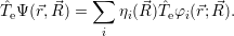
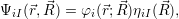
A second approach to the derivation of a molecular wave function was presented by Born more than two decades later [92] (see also [90], Appendix VIII). Instead of a series expansion of the molecular Hamiltonian, this derivation starts with an ansatz-wave function of the form
 | (2.28) |
where the  ;
; ) are the solutions of the electronic Hamiltonian


 ) can be seen as a weighting-factor for the electronic
wave function
) can be seen as a weighting-factor for the electronic
wave function
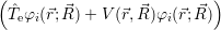
Before the ansatz is inserted into the molecular Schrödinger equation (2.1), it is useful to
apply it to the constituent operators of the associated Hamiltonian (2.2) separately. The
potential operators, which are mere functions of the degrees of freedom, are summed up as
 =
= 


 ) and are applied as
 | (2.29) |
The electronic kinetic energy operator (2.3) acts only on the  ;
; )
)
 | (2.30) |
The application of the electronic Hamiltonian to Ψ(
 ) thus gives
  ) ) | = (  )Ψ( )Ψ(  ) ) | (2.31) |
=  ) )  ; ; ) + ) +   ) ) ; ; ) ) ) ) | (2.32) | |
=  ) ) | (2.33) | |
=  ) ) = =  ) ) | (2.34) |
 ) is again the eigenvalue for
  ;
; ) with respect to
  ;
; ) and the
  ). Using the definition
 | (2.35) |
with
 | (2.36) |
and the product rules for the gradient and the divergence, it is trivial to show that
 | (2.37) |
Applying the Hamilton operator
 | (2.38) |
one arrives at
(  ) = ) = | |||
     = = | (2.39) |
 , yielding the system of
equations
, yielding the system of
equations
 |  )+ )+ | ||
  ) ) | |||
=  ) ) | (2.40) |
 | (2.41) |
with
 | (2.42) |
and
 | = | (2.43) |
| =  | (2.44) |
| =  | (2.45) |
 | =  ; ; ) )  ; ; ) ) + +   ; ; ) )  ; ; ) )  | (2.46) |
 ) is solely due to
If
 | (2.47) |
i.e. the state of the system can be identified by a separate quantum number for the electronic and the vibrational state, respectively. In the more general case where the non-adiabatic part of the Hamiltonian cannot be neglected, the electronic and vibrational quantum numbers are not generally separable and the eigenstates will expand over several electronic states.
There seems to be no established name for the presented approach to the molecular Schrödinger equation. It is sometimes also refered to as Born-Oppenheimer approximation (which is misleading as it is using a completely different derivation), Born-Huang approximation, or Born-ansatz. The non-adiabatic theory not only makes it possible to describe vibronic coupling, but also gives an idea of the conditions under which the adiabatic approximation is reasonable. Following the expressions in [126] and Sec. 3.1.3 of [91], the adiabatic approximation is valid for systems with a large separation between the potential energy surfaces and a weak dependence of the electronic wave functions on the position of the nuclei.
For the derivations in the following sections it is convenient to use a Dirac notation for the Born-Oppenheimer states as
 | (2.48) |
Although one may be tempted to view this wave function as a simple tensor product of wave functions
and employ the usual algebra, this is not possible here due to the parametric dependence of the
electronic state on the vibrational coordinate  . Nevertheless, this notation is often found in literature
and will also be applied in this document where ever it may serve to improve readability.
However, the reader is advised to handle vectors of the form (2.48) with care. To improve
readability somewhat further this document uses a notation that distinguishes between integrals
over the electronic degrees of freedom
. Nevertheless, this notation is often found in literature
and will also be applied in this document where ever it may serve to improve readability.
However, the reader is advised to handle vectors of the form (2.48) with care. To improve
readability somewhat further this document uses a notation that distinguishes between integrals
over the electronic degrees of freedom 
 and over the nuclear degrees of freedom


 .
.
Although in principle a diagonalization of the non-adiabatic Hamiltonian is possible, the resulting
stationary states are not of interest for this work, as we assume transitions between well-defined
electronic states. Indeed, in real-world situations the stationary states corresponding to the
eigenstates of the non-adiabatic Hamiltonian will never be established due to the constant
perturbation from the environment. The influence of the environment is a very complex random
process in nature that cannot be treated, or even formulated, exactly. The theory of vibronic
transitions therefore has to rely on physical intuition and defines the initial and final states of
the transition somewhat heuristically as the initial and final Born-Oppenheimer states
(2.13). It is assumed that initially the electronic subsystem is in a defined state, which is
called  i(
i( )
) in the following. The transition rate to a specific final state
  f(
f( )
) is to be
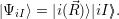
calculated. The vibrational degrees of freedom assumingly have established an equilibrium
with the surrounding lattice, i.e. the probability
is to be
calculated. The vibrational degrees of freedom assumingly have established an equilibrium
with the surrounding lattice, i.e. the probability 

 , given that the electronic system is in state
 | (2.49) |
where
 | (2.50) |
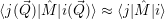
The Born-Oppenheimer states, however, do not diagonalize the non-adiabatic Hamiltonian and thus
will not give rise to stationary states but will decay over time and thus the system will move between
different electronic states. As the off-diagonals in the non-adiabatic Hamiltonian are usually assumed
to be small compared to the diagonal part, the transitions between the electronic states is treated
using first-order time-dependent perturbation theory [98]. Thus, the rate of transition from  Ψ
Ψ to
to
 Ψ
Ψ reads
reads
 | (2.51) |
where the perturbation  is the non-adiabacity operator (2.46).
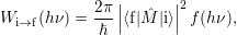
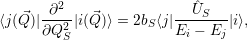
The total rate from  i(
i( )
) to
to  f(
f( )
) is obtained by averaging (2.51) over all possible initial states
 i
i
 and summing over all possible final states
  f
f

 | (2.52) |
where avg
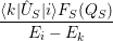
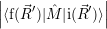
Now that the basic theory of vibronic transitions is laid out, the next important step is the calculation
of the matrix element 
 fF
fF
 f(
f( )
)

 i(
i( )
)
 iI
iI
 . The integration for this matrix element runs over all
electronic and vibrational degrees of freedom and requires the quantum mechanical states of the
electronic and the vibrational system to be known. Especially the latter requirement is impossible to
fulfill exactly for real-world systems, so additional assumptions have to be made. These assumptions
must lead to a model description that captures enough of the basic behavior of the real-world system
to give accurate results yet include only so much complexity that a quantum-mechanical treatment is
still feasible.
. The integration for this matrix element runs over all
electronic and vibrational degrees of freedom and requires the quantum mechanical states of the
electronic and the vibrational system to be known. Especially the latter requirement is impossible to
fulfill exactly for real-world systems, so additional assumptions have to be made. These assumptions
must lead to a model description that captures enough of the basic behavior of the real-world system
to give accurate results yet include only so much complexity that a quantum-mechanical treatment is
still feasible.
The published models for vibronic transitions [127, 128, 129, 91, 130] contain several approximations that simplify the molecular Hamiltonian (2.2) and the corresponding Born-Oppenheimer states. These approximations are described in the following.
As stated above, the molecular Hamiltonian includes the interactions of all electrons and all nuclei.
However, a vibronic transition will usually leave most of the electrons in their respective state thus it
is not necessary to consider them explicitly in the calculation. What has to be considered is their
interactions with the nuclei and with the explicitly treated electrons (usually only one). The former
interactions together with the Coulomb repulsion 
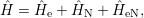 | (2.53) |
where
 | (2.54) |
acts only on the nuclei. The details of
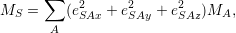
Another important approximation concerns the potentials 

 | (2.55) |
it is always possible to define a coordinate system 
 =
= 
 | (2.56) |
The eigenvalue Λ
 | (2.57) |
using the mass
 | (2.58) |
as in a classical picture this leads to a nuclear motion that is composed of uncoupled harmonic modes
with the frequencies
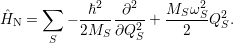 | (2.59) |
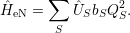
An additional assumption that is always employed but rarely stated explicitly is that the
electron-phonon interaction  [129, 131]. In this case the interaction Hamiltonian can be written as
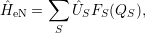 | (2.60) |
where
The transition rate is now determined from (2.52), with the wave functions in the modal coordinate system
 | (2.61) |
and the non-adiabacity operator
 | =  | (2.62) |
 | =    ) )    ) )    ) )    ) )  | (2.63) |

 )
) are the solutions of the equation
 | (2.64) |
In addition to the  using a perturbation expansion based on the (
 -independent) solutions of the electronic
Hamiltonian
-independent) solutions of the electronic
Hamiltonian
 | (2.65) |
An exception is the work of Kubo [128], which uses a highly idealized defect wave function. In the
Condon approximation or adiabatic approximation (not to be confused with the adiabatic
Born-Oppenheimer approximation), the  -dependence of the electronic wave functions is obtained
from first-order perturbation theory, i.e.
-dependence of the electronic wave functions is obtained
from first-order perturbation theory, i.e.
  ) ) | =   + +    | ||
=   + +    | (2.66) | ||
 ) ) | =     | ||
=     | (2.67) |
  ) )   ) ) | =     | ||
+           + +           | |||
| + second order terms | (2.68) |
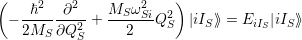
The perturbation expansion of the energy has an important consequence for the vibrational system, as in the employed Born-Oppenheimer approximation the energy levels act as a potential for the nuclei. The vibrational part of the problem now reads
 | (2.69) |
This Hamiltonian is a sum of independent operators for every phonon mode which is solved by the wave function [98]
 | (2.70) |
with the corresponding energy
 | (2.71) |
and the constituents 

 and
and
 | (2.72) |
In essence, this result makes the true separation of the phonons possible, which is of importance for
the following considerations. The quantum state of the vibrational system
In most publications, the coupling function  ) is a linear expression in the modal coordinates [130]
 | (2.73) |
where
Inserting the linear relation for
 | (2.74) |
with
 | (2.75) |
The resulting modal wave functions are harmonic oscillator wave functions [139]
   | = | (2.76) |
| = | (2.77) | |
=  | (2.78) | |
=   | (2.79) |
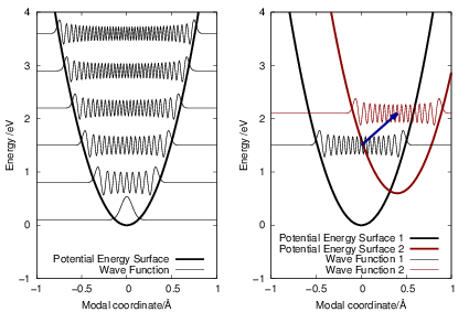
| Figure 2.6: | Potential energy surfaces and the corresponding vibrational wave functions for
one mode in the linear coupling approximation. |
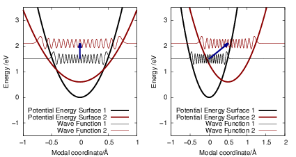
| Figure 2.7: | Potential energy surfaces and vibrational wave functions for a transition in the
quadratic coupling |
In addition to the linear coupling approximation, some works also investigate systems with purely
 | (2.80) |
As shown in Fig. 2.7, contrary to the linear coupling, the quadratic coupling does not change the equilibrium coordinate of the mode but the oscillation frequency, leading to a vibrational Schrödinger equation of the form
 | (2.81) |
with
 | (2.82) |
The vibrational wave functions thus assume the form
   | = | (2.83) |
| = | (2.84) |
 | (2.85) |
and upon a transition between two electronic states both the equilibrium position and the oscillation frequency of the phonon modes change, yielding the vibrational Schrödinger equation
 | (2.86) |
with
=  | (2.87) | |
=  | (2.88) | |
=   | (2.89) |
Line shapes are a concept originating from the field of optical spectroscopy. As an introduction to the
concept, we take a look at the first quantitative theory for the multi-phonon transitions of a
point-defect derived by Huang and Rhys [127] in 1952 for the F-Center in potassium bromide. The
first part of that work is dedicated to a transition induced by incident radiation. In these transitions,
the dominant perturbation arises from the polarization operator  and not from the non-adiabacity
operator
and not from the non-adiabacity
operator  in (2.52). It is safe to assume that
  acts only on the electrons, again due to the
comparably large mass of the nuclei. In the Condon approximation (2.68) the corresponding matrix
element reads
acts only on the electrons, again due to the
comparably large mass of the nuclei. In the Condon approximation (2.68) the corresponding matrix
element reads
  ) )    ) ) = = |      | ||
+            | |||
           | (2.90) |


 . Consequently the sums in (2.90) can be neglected
and the electronic matrix element is approximately independent of the position of the
nuclei.
. Consequently the sums in (2.90) can be neglected
and the electronic matrix element is approximately independent of the position of the
nuclei.
 | (2.91) |
This is known as the quantum mechanical Franck-Condon principle [127, 91]. It is important to stress
that the  -independence only concerns the matrix element but not its constituents. In this
case, the electronic matrix element in (2.51) can be taken out of the integration over
-independence only concerns the matrix element but not its constituents. In this
case, the electronic matrix element in (2.51) can be taken out of the integration over  ,
yielding
,
yielding
 | (2.92) |
In essence, this describes the transition as an electronic matrix element with vibrational selection
rules. The factors 
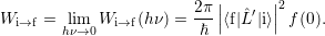
Inserting this matrix element into (2.52) results in the expression [117]
 | (2.93) |
where
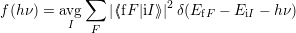 | (2.94) |
is the
While the Franck-Condon principle is easy to justify for optical matrix elements using the Condon
approximation, the above argument completely fails for the non-adiabacity operator (2.63) which
contains the electronic matrix elements 


 and
and 


 that do not
induce a direct transition. Using the interaction (2.85), the Condon approximation for these matrix
elements gives with (2.66)
that do not
induce a direct transition. Using the interaction (2.85), the Condon approximation for these matrix
elements gives with (2.66)
 | (2.95) |
and
 | (2.96) |
and the transition matrix element reads with (2.63)
     ) )    ) )    | =        | (2.97) |
       | = | (2.98) |
=       | (2.99) | |
=     + +        + 2 + 2       | (2.100) |
Inserting (2.70) for the vibrational wave functions gives
 | (2.101) |
This result is interesting as it shows that each mode contributes a Frank-Condon factor to the matrix
element of every other mode. The vibrational part is determined by the change of the potential energy
surface between the states, which is caused by the diagonal part of the electron-phonon
coupling Hamiltonian 


 , see (2.67). The electronic matrix element, on the other hand,
arises from the off-diagonal elements
, see (2.67). The electronic matrix element, on the other hand,
arises from the off-diagonal elements 


 . As the diagonals and the off-diagonals of
the coupling operator need not be related to each other, there is no direct link between
the contribution of a mode to the electronic matrix element and its contribution to the
vibrational part. In the literature, modes contributing to the electronic matrix element are
called
. As the diagonals and the off-diagonals of
the coupling operator need not be related to each other, there is no direct link between
the contribution of a mode to the electronic matrix element and its contribution to the
vibrational part. In the literature, modes contributing to the electronic matrix element are
called
The target of the present work is to extract relevant parameters for the non-radiative transitions
from atomistic calculations. Although the parameters 


 required for the promoting contribution due to the ill-defined or inaccurate wave
functions in the available electronic structure methods. Under this viewpoint, an approach
to calculate the non-radiative transition rate using the accurate operator (2.98) appears
unreasonable due to the inaccuracy of the underlying model system. We therefore assume that all
modes in our system are purely accepting modes, which enter the transition rate only
through the Franck-Condon factors
required for the promoting contribution due to the ill-defined or inaccurate wave
functions in the available electronic structure methods. Under this viewpoint, an approach
to calculate the non-radiative transition rate using the accurate operator (2.98) appears
unreasonable due to the inaccuracy of the underlying model system. We therefore assume that all
modes in our system are purely accepting modes, which enter the transition rate only
through the Franck-Condon factors 


 and the conservation of energy. We assume a
perturbation operator
and the conservation of energy. We assume a
perturbation operator 
 . Just as
  ,
, 

 | (2.102) |
This approach is well compatible with published works which either apply the Frank-Condon principle directly to the non-adiabacity operator [127, 117, 131, 142] or where the perturbation does not arise from the non-adiabacity operator but instead from an applied field [143, 144].
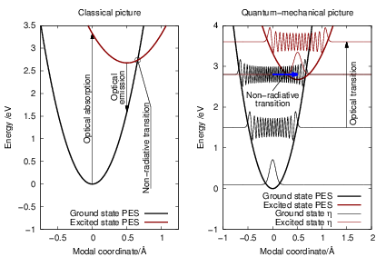
| Figure 2.8: | A schematic configuration-coordinate diagram illustrating vibronic transitions
in a classical and a quantum mechanical picture. In the classical picture |
As for the barrier hopping transitions in Sec. 2.8, it is also possible to formulate a theory for vibronic transitions that treats the nuclei as classical particles [129, 117]. Several semi-classical approaches have been published over the years, especially for the estimation of reemission probabilities [117] or correlated hopping [116]. In the present work, non-Markovian behavior is not assumed to be relevant, so the theory is again derived using the assumption of thermal equilibrium.
As above, we derive the non-radiative transition from an optical transition by letting the optical
energy approach zero. In this approach, the transition between the electronic Born-Oppenheimer wave
functions  i(
i( )
) and
and  f(
f( )
) proceeds via the optical matrix element
  . For any position
  of the
nuclei, one can now again employ time-dependent perturbation theory to calculate the transition rate
as
of the
nuclei, one can now again employ time-dependent perturbation theory to calculate the transition rate
as
 | (2.103) |
Again following just the same considerations as before, we assume that the nuclear degrees of
freedom are in thermal equilibrium and can be described by classical statistical physics. The
probability to find the system in electronic state  i
i at a certain configuration
  is hence given
by
is hence given
by
 ) ) | = 
| (2.104) |
=  
 | (2.105) |
=    
  | (2.106) | |
= 
   d d | (2.107) |
=   | (2.108) | |
= 
 d d | (2.109) |

Now that the chemical states and reactions are defined and we have obtained rates for the reactions
from the explained microscopic theories, we can calculate the time evolution of the chemical system
from the chemical master equation (2.20). As explained above, this equation is a stochastic differential
equation which assigns a probability to any state vector  , given that
  =
= 


 is generated using pseudo-random numbers. The SSA does not have any algorithmic
parameters and is a mathematically exact description of the system defined by the states and
reaction channels [114]. The moments of the probability distribution
is generated using pseudo-random numbers. The SSA does not have any algorithmic
parameters and is a mathematically exact description of the system defined by the states and
reaction channels [114]. The moments of the probability distribution 
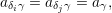
Most chemical systems are constructed of a large number Θ of similar sub-systems with a small number of states Ω, for example a number Θ of well-separated doping atoms within a semiconductor device which can exist in a number Ω of different charge states. The chemical state of the total system can in principle be constructed from all the states of the subsystems, i.e.
 | (2.110) |
For every subsystem 


In a situation like this a given observable will usually be unable to separate these sub-systems. For
instance for the transport characteristics of a semiconductor device it is irrelevant
 | (2.111) |
the chemical state of the total system can be reformulated, considering only the numbers of
subsystems 
 | (2.112) |
the state change vectors will only operate on the numbers
 | (2.113) |
corresponding to the probability per unit time that 
 | (2.114) |
which is the probability per unit time that any two of the
 | (2.115) |
which corresponds to the probability that
Bimolecular reactions usually emerge in situations when at least one of the specimens is able to
move, giving it access to different reaction partners. A mathematical description of the form (2.114) or
(2.115) implies, that the reaction probability is the same for every pair of reactants, i.e. a
homogeneous distribution of the reacting specimens within the volume associated with the chemical
system. This condition is commonly referred to as the system being
As stated above, it is quite common that observables only determine how many constituents of a
chemical system have assumed a certain state, or equivalently how many specimens of a certain species
exist in that system. Usually the most interesting quantities for a chemical system in number
representation is thus the development of the
 | (2.116) |
which corresponds to the first moment of the probability distribution
To obtain these averages from the SSA one has to take the average of several simulation runs, which
is usually a quite time-consuming task. Especially if there are very fast reactions or a large number of
particles in the system, the simulation of longer time-ranges quickly becomes unfeasible using this
approach. A computationally more efficient approach is to directly calculate the dynamics of the
average values. For convenience we introduce the average number vector  =
=  . The time evolution
of
. The time evolution
of  is calculated from
 | (2.117) |
The substitution of the right side of (2.20) for the derivative of
 | (2.118) |
For the case of unimolecular reactions (2.113), whose propensity functions are linear in  , it is trivial
to show that
, it is trivial
to show that  =
= 
 , which leads to the popular description using reaction rate
equations
, which leads to the popular description using reaction rate
equations
 | (2.119) |
Due to their efficiency and simplicity, reaction rate equations are a popular method to describe reactive systems. However, one has to be aware that this description is only exact if all the reactions in the system are unimolecular. Nevertheless, reaction rate equations are also commonly used for systems with bimolecular reactions and even reactive-diffusive systems, as in the reaction-diffusion model for NBTI. The consequences and inadequacies of this approach are discussed in Chap. 3.
As a final remark, it is common not to use the number-representation of  . Instead, the number of
particles is usually normalized to the volume of the system, leading to a formulation based on
. Instead, the number of
particles is usually normalized to the volume of the system, leading to a formulation based on


